Look, it’s Anscombe’s quartet on steroids!
Q: What is Anscombe’s quartet?
A: Anscombe’s quartet is a set of four datasets, each with 11 observations on two variables x and y, that all have (nearly) identical descriptive statistics but appear very different when graphed. The datasets all have approximately the same means (for both X and Y), variances (for both X and Y), correlations, linear regression lines, and coefficients of determination. But they look like this when graphed:

The idea behind the quartet of datasets, developed by Francis Anscombe in 1973, was to demonstrate the importance of graphing/visualizing your data in addition to just looking at its summary values.
One thing that’s not known about these datasets is exactly how Anscombe created them. But a 2017 paper titled “Same Stats, Different Graphs: Generating Datasets with Varied Appearance and Identical Statistics through Simulated Annealing” shows a method for creating differently “shaped” datasets that all have the same summary values. In this paper, the “Datasaurus Dozen” are produced: a set of 12 differently-shaped datasets (when graphed) that have the same summary stats. The paper talks about a method used to create these datasets.
It’s super cool and very interesting. Check it out here!
NEEEEEEEEEEEERDS! (Actually, Skittles)
Today I found this blog post, which is a follow-up to another blog post talking about how many bags of Skittles would need to be observed before two identical packs (same number of candies, same color distribution) were discovered.
In this follow-up post, the author also looks at the overall distribution of the colors across the packs and finds the following:

(Image from here)
They remark: “The most common and controversial question asked about Skittles seems to be whether all five flavors are indeed uniformly distributed…I leave it to an interested reader to consider and analyze whether this departure from uniformity is significant.”
Well, I am an interested reader, so here we go.
We’re going to test the claim that the flavors* are uniformly distributed (by stating that the proportions of each of these five flavors are equal) against the claim that the flavors are not uniformly distributed (by stating that at least one proportion differs from the others).

Let’s use p-value = 0.05.
The author has graciously made their data available to the public, so I snagged it up and got the following information:

Applying a chi-square goodness-of-fit test, we get the following results:

Since our p-value of 0.001 < 0.05, we reject H0 and conclude that at least one of the above proportions differs from the expected 0.20 under the null hypothesis. This means that statistically, the proportions are significantly different.
…I should be getting stuff ready for the end of the semester. Or working on my NaNo. Why did I do this?
*I’m using color rather than flavor, since a) “red” is easier to type than “strawberry” and b) candy flavors such as these are MEANINGLESS TO MY BROKEN NOSE
Want Some Data?
Hello again, all.
So it occurred to me that I have thousands of data points in the form of my walking data that I haven’t shared in any form other than yearly summaries and graphs.
So I’ve decided to post a link to my entire Excel file of walking data since moving to Calgary. You know, for anyone who needs data or wants to analyze it or who just thinks I’m making it all up.*
So here ya go! Nerd it up.
*I’m not. Do you know how lazy I am? It would take a lot of effort to realistically fake that much data.
Heights
Heyooooo so I was looking for some new data to update one of my STAT 213 note sets and I decided to use the on-record heights for 500 baseball players. We’re learning about types of graphs (boxplots, histograms, etc.) and ways of describing the shape of graphs (symmetric, skewed, etc.) so I thought hey, let’s plot these heights and see what we get.
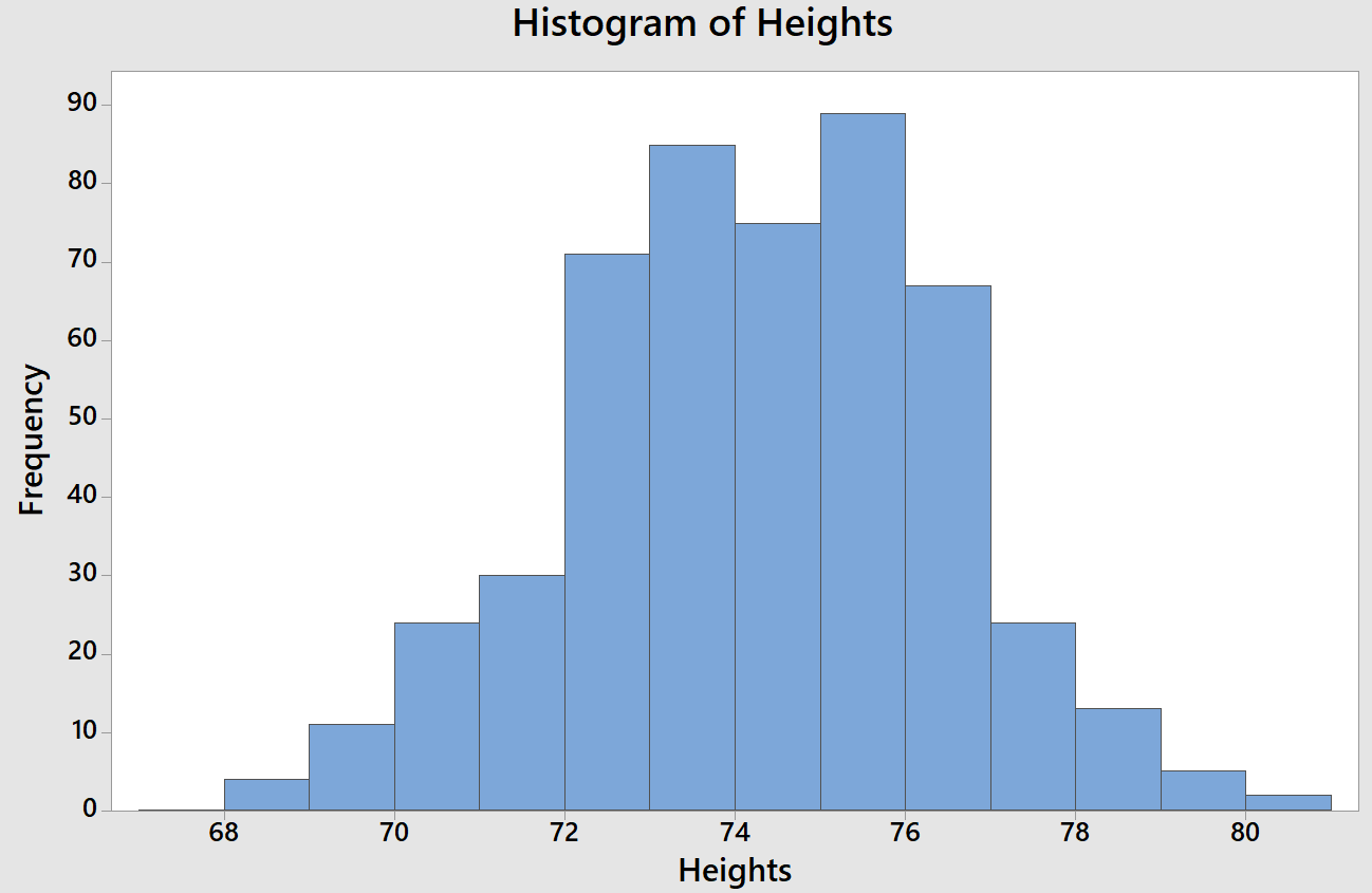
UHHHH, have you ever seen such a perfect bell-curve shape for actual data?
But here’s where it’s interesting to also look at not only the numeric summary but other plots as well. The boxplot actually shows two outliers (two players at 80 inches tall).

So that’s interesting as well.
Anyway. Just thought this was a super pretty distribution and I have no life so I wanted to share this with y’all.
Baseball Stat Party Fun Time
A fun project!
At the end of the regular baseball season, you can see how many wins each team got out of the total number of games they played, and then rank the teams by their performance (who had the most wins, the second most wins, etc.).
What I want to do is see how this “real” data correlates with how many wins each team would get if they scored their average number of runs per game in every single game they played. For example, if the Mariners score an average of 4.74 runs per game, how many of their games would they have won by scoring 4.74 runs in each of those games?
The process:
- Record each team’s average runs per game (I’ll call this “RPG”) (from here)
- Sort teams from highest to lowest RPG
Now, if a team A has a higher RPG than team B, that would mean that A would win every game they play against B. So the next step was to make a grid like this and fill in the number of times each pair of teams played each other.
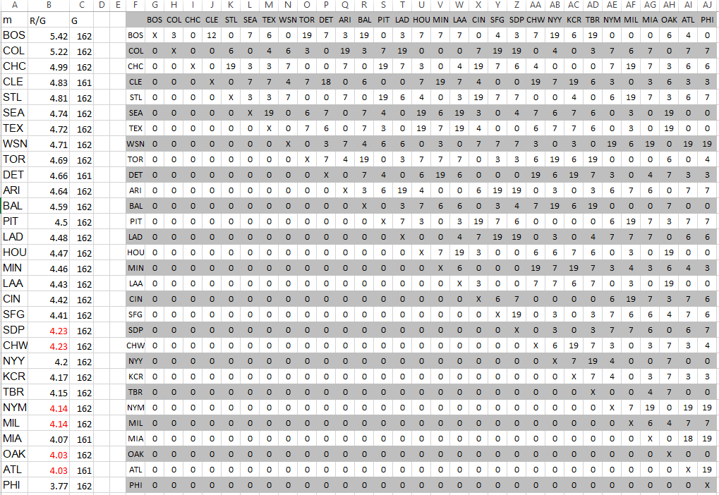
Boston has a higher RPG than the Rockies (5.42 and 5.22, respectively). So that means Boston would score 5.42 runs and the Mariners would score 5.22 runs in every game they played against each other. So of the 7 games played where these two teams faced each other, that would mean that Boston would win all of them.
I used this logic for all pairings (numbers of games per pair was obtained from here), then summed across the rows to get the “predicted” number of wins based on RPG alone.
How do they compare for the 2016 season?

Boston (highest RPG) would win every game they played; The Phillies (lowest RPG) and the Athletics (bad luck) would lose every game they played. Bummer.
Correlation of RPG-predicted games won and actual games won: 0.640
Correlation of team rankings based on RPG-predicted games won and actual games won: 0.683
Interesting!
Biostatistics Ryan Gosling
Haha, these are great.
I’m surprised Nate didn’t hear me laughing like an idiot at these at 4:00 in the morning.
Favorites:


The end.
Deriving the Negative Binomial Probability Mass Function
Today is going to kind of be a continuation off of yesterday’s post about the binomial. Today, however, we’re going to focus on the negative binomial and how you can derive the formula for the negative binomial from the binomial itself. Let’s do this with an example:
Scenario: A recent poll has suggested that 64% of Canadians will be spending money – decorations, Halloween treats, etc. – to celebrate Halloween this year. What is the probability that the 13th Canadian random chosen is the 6th to say they will be spending money to celebrate Halloween?
Solving it the Binomial Way
This sounds like a binomial-type question, right? So your first thought might be as follows:
“I need to have a total of 6 ‘successes’ out of a total of 13 people asked. So n = 13, p = 0.64, and I’m looking for P(X = 6). I can apply the binomial formula like this:”
![]()
This is how we applied the binomial formula in a similar problem yesterday. But if you look closer at this question specifically, this isn’t quite asking for something that we’ve seen the binomial used for. The above binomial calculation works if you need a total of 6 successes from 13 trials and it doesn’t matter in which order they came.
This question, though, is stating that that 13th trial needs to be one of the successes—more specifically, it needs to be the 6th one. So how can we approach that?
Let’s divide the problem into two easier-to-solve parts. Based on the question, we know that the 13th trial needs to be a success. So ignore it for a second. If we ignore the 13th trial, we’re also ignoring the 6th success.
So what we’re left with is 12 trials and 5 successes.
The question doesn’t say anything about these 12 trials other than that 5 of them have to be successes. This allows us to use the binomial formula to figure out the probability that 5 of the 12 are successes: n = 12, p = 0.64, and we’re looking for P(X = 5):
![]()
That takes care of the first 12 trials. Let’s go back to the 13th one. We know, from the question, that the 13th one needs to be a success. We can find this easily: since it’s just one trial, and we know the trials are all independent and all have the same probability of success, the probability of this 13th trial being a success is just equal to 0.64, our probability of success.
Now we’ve got the two parts: the first 12 trials and the 13th trial. So how do we put this together to find the answer to the question? As I just mentioned, all the trials are all independent, so we can just multiply their probabilities:
![]()
There’s your answer!
Solving it the Negative Binomial Way
The negative binomial probability model is generally used to answer the question, “what is the probability that it will take me n trials to get s successes?”
Let n = the number of trials and s = the number of successes. To find P(X = n), or the probability that you’ll need n trials to get to a specified s number of successes, you find the following:
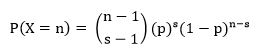
Let’s plug in our values from our question, which is asking for P(X = 13), so n = 13 and s = 6:
![]()
If we break up that 0.646 into (0.645)(0.641), you’ll notice that this equation is exactly the same as the one we used when solving this the binomial way.
![]()
This part was from our first 12 trials, this part was from our 13th trial and knowing it was a success. So if you solve this the binomial way, you actually are solving it using the negative binomial equation!
Deriving the Binomial Probability Mass Function
Today I want to talk about binomial random variables. Specifically, I want to talk about how you can “derive” the binomial probability mass function (pmf) using a simple example.
I want to discuss these things in a way that someone who is completely unfamiliar with statistics can understand them, so let’s start from the beginning!
- What is a binomial random variable?
- What is a probability mass function?
- What is the probability mass function for a binomial random variable?
- How can you “derive” this probability mass function from a simple example?
- What is a binomial random variable?
You can think of a binomial random variable as something that counts how often a particular event occurs in a fixed number of trials. In order for a variable to be a binomial random variable, the following conditions must be met:
- Each trial must be performed the same way and must be independent of one another
- In each trial, the event of interest either occurs (a “success”) or does not (a “failure”) (in other words, there must be a binary outcome in each trial)
- There are a fixed number, n, of these trials
- In each of the n trials, the probability of a success, p, is the same.
Here are some good “basic” examples of binomial random variables:
- Define a “success” as getting a “heads” on a coin flip. If you flip 10 coins and let X be the number of heads you get from those 10 flips, X is a binomial random variable (n = 10, p = 0.5)
- Define a “success” as rolling a 5 on a 6-sided die. If you roll a die 20 times and let X be the number of times you roll a 5, then X is a binomial random variable (n = 20, p = 1/6)
- The probability of any given person being left-handed is 0.15. If you randomly ask 50 people if they are left-handed or not, and let X be the number of people who are left-handed out of the 50, then X is a binomial random variable (n = 50, p = 0.15).
As you can see, there are really two values we need to know in order to define something as a binomial random variable (which, in reality, is defining the shape of the binomial distribution from which that random variable comes): n, the number of trials, and p, the number of successes. If X is a binomial random variable, we can express this as X~binom(n,p). This is read as “X follows a binomial distribution with n trials and a probability of success p.” In our previous three examples, we could express the X’s as follows:
- X~binom(10,0.5)
- X~binom(20,1/6)
- X~binom(50,0.15)
- What is a probability mass function?
A probability mass function (pmf) is a lot less scary than it sounds. It is simply a function that gives the probability that a (discrete) random variable is exactly equal to some value. For example, suppose X is our random variable. Let x represent a specific value that X could assume. A pmf for X could give us P(X = x), or the probability that X is equal to that specific value x.
- What is the probability mass function for a binomial random variable?
Let X be a binomial random variable. To find the probability that X equals a specific value x, we use the following formula:
![]()
where n is the number of trials, p is the probability of success, and
- How can you “derive” this probability mass function from a simple example?
This pmf might look a little complicated. However, we can understand it and how it comes about by looking at a simple example and “working backwards” to get to the above pmf formula. So let’s do it!
Suppose you roll a fair die four times. Let X be the number of times you roll a 1. You want to find the probability of rolling exactly three 1s.
In this example, the number of trials is the number of rolls. So n = 4. The probability of success is the probability of rolling a 1 on any given roll. So p = 1/6. And what we want to find is the probability that exactly three of the four rolls will result in a success. So we want P(X = 3).
Let’s see if we can figure this out without the formula.
We want the probability of getting exactly three successes out of the four rolls, or P(three successes). Another way of stating this is that we want P(success and success and success and failure), or that we want three successes and one failure. Don’t worry about the order yet; we’ll deal with that later.
So. We know that the probability of success on any one roll is 1/6, which means that the probability of failure on any one roll is 5/6. We also know that the rolls are independent of one another, as the outcome of one roll does not affect the outcome of another (e.g., rolling a 5 on the first roll will not affect the outcome of the second roll).
Because of this independence, our calculation of P(success and success and success and failure) is just going to be the probabilities of each of the four outcomes multiplied by each other, or
![]()
In our example, this is
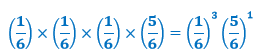
Notice that this is the
![]()
part of the pmf formula when x = 3 and n = 4. This is the part that gives us the probability of three successes out of four trials. However, we’re not done yet! We also need to take into account the fact that these three successes and one failure can happen in different orders. Specifically, if we denote a success as “S” and a failure as “F,” these can occur in the following orders:
SSSF
SSFS
SFSS
FSSS
That is, there are four different ways we can get three successes and one failure when n = 4. So what we need to do now is combine this with our previous calculation above to get

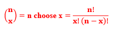
That 4 is actually the number of combinations of three successes and one failure we can get when n = 4. Another way we could calculate this without writing out all the possible combinations? Use this formula:
![]()
Specifically:
![]()
Our final calculation, then, is

So the probability of rolling exactly three 1s out of four rolls is 0.01543, and we can see that in our process of figuring this out, we’ve actually “derived” our binomial formula of

Cool, huh?
Week 42: Goodman and Kruskal’s Gamma
Let’s keep going with measures of correlation and talk about Goodman and Kruskal’s gamma today!
When Would You Use It?
Goodman and Kruskal’s gamma is a nonparametric test used to determine, in the population represented by a sample, if the correlation between subjects’ scores on two variables is some value other than zero.
What Type of Data?
Goodman and Kruskal’s gamma requires both variables to be ordinal data.
Test Assumptions
No assumptions listed.
Test Process
Step 1: Formulate the null and alternative hypotheses. The null hypothesis claims that in the population, the correlation between the scores on variable X and variable Y is equal to zero. The alternative hypothesis claims otherwise (that the correlation is less than, greater than, or simply not equal to zero).
Step 2: Compute the test statistic, a z-value. To do so, Goodman and Kruskal’s gamma, G, must be computed first. The following steps must be employed:
- Arrange the data into an ordered r x c contingency table, with r representing the number of levels of the X variable and c representing the number of levels in the Y variable. The first row represents the category that is lowest in magnitude on the X variable and the first column represents the category that is lowest in magnitude on the Y variable. Within each cell of the table is the number of subjects whose categorization on the X and Y variables corresponds to the row and column of the specified cell.
- Calculate nc, the number of pairs of subjects who are concordant with respect to the ordering of their scores on the two variables. This is done as follows, starting at the upper left-hand corner of the table: for each cell, determine the frequency of that cell, then multiply that frequency by the sum of all the frequencies of all cells that fall both below it and to the right of it. The sum of these products is nc.
- Calculate nd, the number of pairs of subjects who are discordant with respect to the ordering of their scores on the two variables. This is done as follows, starting at the upper right-hand corner of the table: for each cell, determine the frequency of that cell, then multiply that frequency by the sum of all the frequencies of all cells that fall both below it and to the left of it. The sum of these products is nd.
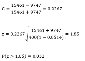
- Compute G as follows:
![]()
The test statistic itself is calculated as:

Where N is the total number of subjects whose scores are recorded in the contingency table.
Step 3: Obtain the p-value associated with the calculated z-score. The p-value indicates the probability of observing a correlation as extreme or more extreme than the observed sample correlation, under the assumption that the null hypothesis is true.
Step 4: Determine the conclusion. If the p-value is larger than the prespecified α-level, fail to reject the null hypothesis (that is, retain the claim that the correlation in the population is zero). If the p-value is smaller than the prespecified α-level, reject the null hypothesis in favor of the alternative.
Example
Let’s see if there’s a relationship between stars (3, 4, or 5) and what I consider to be my favorite four genres: electronic, pop, alternative, and rock (in that order). Let X be the song’s genre and let Y be the number of stars received by the song. The following is an ordered contingency table of a sample of 400 songs (100 of each genre).

I suspect a positive correlation between ranked favorite genres and stars. Here, n = 400 and let α = 0.05.
H0: γ = 0
Ha: γ > 0
The calculations for nc and nd:

And G and the test statistic:
Since our calculated p-value is smaller than our α-level, we reject H0 and conclude that the correlation in the population is significantly greater than zero.
Week 40: Kendall’s Tau
Let’s do another measure of correlation, shall we? Kendall’s tau!
When Would You Use It?
Kendall’s tau is a nonparametric test used to determine, in the population represented by a sample, if the correlation between subject’s scores on two variables equal to a value other than zero.
What Type of Data?
Kendall’s tau requires both variables to be ordinal data.
Test Assumptions
No assumptions listed.
Test Process
Step 1: Formulate the null and alternative hypotheses. The null hypothesis claims that in the population, the correlation between the ranks of subjects on variable X and variable Y is equal to zero. The alternative hypothesis claims otherwise (that the correlation is less than, greater than, or simply not equal to zero).
Step 2: Compute the test statistic, a z-value. To do so, Kendall’s tau must be computed first. The following steps must be employed:
- Arrange the data by the ranking on the X variable (smallest to largest ranking).
- Begin with the first Y rank corresponding to the first (smallest) X rank. If the Y rank for the smallest X ranking is larger than any Y ranks corresponding to any of the other X ranks, note it with a “D” for discordant. If the Y rank for the smallest X ranking is smaller than any Y ranks corresponding to any other X ranks, note it with a “C” for concordant.
- Once this is done for all comparisons for the first Y rank, move on to the second Y rank and repeat steps 2 and 3 until all ranks are considered.
- For each Y rank, sum the number of Cs and the number of Ds. The sum of all the Cs across all rankings gives you nC, the total number of C entries, and the sum of all the Ds across all rankings gives you nD, the total number of D entries.
Compute Kendall’s tau as follows:
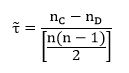
where nC and nD are as defined above and n is the total number of data points in the sample.
The test statistic itself is calculated as:

Step 3: Obtain the p-value associated with the calculated z-score. The p-value indicates the probability of observing a correlation as extreme or more extreme than the observed sample correlation, under the assumption that the null hypothesis is true.
Step 4: Determine the conclusion. If the p-value is larger than the prespecified α-level, fail to reject the null hypothesis (that is, retain the claim that the correlation between the ranks in the population is zero). If the p-value is smaller than the prespecified α-level, reject the null hypothesis in favor of the alternative.
Example
I want to see if there’s a correlation between my ranking of 12 of my songs from 2009 and the ranking of those 12 same songs in 2016. Let X be the ranking in 2009 and Y be the ranking in 2016. Let’s use α = 0.05. I actually have no idea if this will end up a positive or negative correlation, so let’s go with the most general hypotheses:
H0: τ = 0
Ha: τ ≠ 0
The table below shows the rankings of the 12 songs for 2009 and 2016, as well as the method to obtain the sums of Cs and sums of Ds.
nC = 42 and nD = 24
Kendall’s tau and the test statistic:

Since our calculated p-value is larger than our α-level, we fail to reject H0 and conclude that the correlation between the ranks in the population is not significantly different from zero.
Week 39: Spearman’s Rank-Order Correlation Coefficient
Let’s talk about the Spearman’s rank-order correlation coefficient today!
When Would You Use It?
The Spearman’s rank-order correlation coefficient is a nonparametric test used to determine, in the population, if the correlation between values on two variables is some value other than zero. More specifically, it is used to determine if there is a significant linear relationship between the two variables.
What Type of Data?
The Spearman’s rank-order correlation coefficient requires both variables to be ordinal data.
Test Assumptions
No assumptions listed.
Test Process
Step 1: Formulate the null and alternative hypotheses. The null hypothesis claims that in the population, the correlation between the scores on variable X and variable Y is equal to zero. The alternative hypothesis claims otherwise (that the correlation is less than, greater than, or simply not equal to zero).
Step 2: Compute the test statistic, a t value. To do so, Spearman’s rank-order correlation coefficient, rs, must be computed first. The following steps must be employed:
- Rank both variables in order from smallest to largest, assigning a value of “1” to the smallest value for each variable, a “2” for the second-smallest value for each variable, etc.
- For each pair of observations (that is, for each paired value of X and Y, compute di, the difference between the ranked values of Xi and Yi.
- Compute di2, the squared difference of the ranks of Xi and Yi.
- Compute rs as follows:

The test statistic itself is calculated as:

which is a t-value with degrees of freedom n – 2. Here, rs is the Spearman rank-order correlation coefficient and n is the sample size.
Step 3: Obtain the p-value associated with the calculated z-score. The p-value indicates the probability of observing a correlation as extreme or more extreme than the observed sample correlation, under the assumption that the null hypothesis is true.
Step 4: Determine the conclusion. If the p-value is larger than the prespecified α-level, fail to reject the null hypothesis (that is, retain the claim that the correlation in the population is zero). If the p-value is smaller than the prespecified α-level, reject the null hypothesis in favor of the alternative.
Example
Let’s look at a random selection of 10 of my songs and see if there is a significant correlation between the number of stars a song has (its “rating”) and the number of times it has been played (its “playcount”). Let the X variable be the song’s rating and the Y variable be its playcount. I suspect a positive correlation between rating and playcount (or else my rating system is highly flawed!) Here, n = 10 and let α = 0.05.
H0: rs = 0
Ha: rs > 0
The following table shows the raw data and the rankings needed to compute rs.

Here Rx and Ry represent the ranks of X and Y, respectively, d represents the difference Rx – Ry, and d2 is the squared differences.

Since our calculated p-value is smaller than our α-level, we reject H0 and conclude that the correlation in the population is significantly greater than zero.
Week 38: The Tetrachoric Correlation Coefficient
Let’s talk about another measure of association today: the tetrachoric correlation coefficient!
When Would You Use It?
The tetrachoric correlation coefficient is a parametric test used to determine, in the population, if the correlation between values on two variables is some value other than zero. More specifically, it is used to determine if there is a significant linear relationship between the two variables.
What Type of Data?
The tetrachoric correlation coefficient requires both variables to be interval or ratio data, but also that both of them have been transformed into dichotomous nominal or ordinal scale variables.
Test Assumptions
- The sample has been randomly selected from the population it represents.
- The underlying distributions for both the variables involved is assumed to be continuous and normal.
Test Process
Step 1: Formulate the null and alternative hypotheses. The null hypothesis claims that in the population, the correlation between the scores on variable X and variable Y is equal to zero. The alternative hypothesis claims otherwise (that the correlation is less than, greater than, or simply not equal to zero).
Step 2: Compute the test statistic, a z-value. To do so, the actual correlation coefficient, rtet, must be calculated first. This calculation requires the information on the variables X and Y to be displayed in a table such as the following:
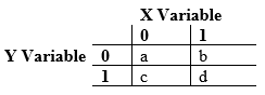
Where “0” and “1” are the coded values of the dichotomous responses for X and Y, and the values a, b, c, and d represent the number of points in the sample that belong to the different combinations of 0 and 1 for the two variables.
Once the table is constructed, rtet is computed as follows:

To compute the z-statistic, the following equation is used:
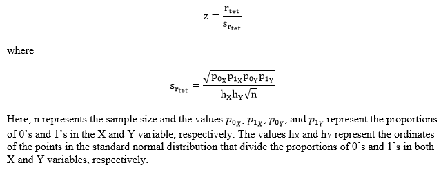
To obtain h for each variable, first find the z-value that delineates the point on the normal curve for which the proportion of cases corresponding to the smaller of p0 and p1 falls above that point and the larger of the two proportions p0 and p1 falls below. This table lists the ordinates for specific z-scores.
Step 3: Obtain the p-value associated with the calculated z-score. The p-value indicates the probability of observing a correlation as extreme or more extreme than the observed sample correlation, under the assumption that the null hypothesis is true.
Step 4: Determine the conclusion. If the p-value is larger than the prespecified α-level, fail to reject the null hypothesis (that is, retain the claim that the correlation in the population is zero). If the p-value is smaller than the prespecified α-level, reject the null hypothesis in favor of the alternative.
Example
Let’s look at the exam grades for one of the old STAT 213 classes. I want to see if there is a significant correlation between the grades on midterm 1 and midterm 2 as far as whether they got a grade higher than a C+. I will code a grade higher than a C+ as 1 and a grade equal to or lower than a C+ as a 0. Let the X variable be the grade on the first midterm, and the Y variable be the grade on the second midterm. I suspect a negative correlation between X and Y, since a lot of students who did poorly on the first midterm either dropped the class or worked really hard to do well on the second one. Here, n = 105 and let α = 0.05.
H0: ρtet = 0
Ha: ρtet > 0
The following table shows the distribution of the 0’s and 1’s for these two variables:

Computations:
First, let’s find the h values. For midterm 1, p0 = 0.18 and p1 = 0.82. The z-score for which 0.82 of the distribution falls below and 0.21 of the distribution falls above is 0.92. The ordinate, h, of this value is 0.2613 according to the table. For midterm 2, p0 = 0.31 and p1 = 0.69. The z-score for which 0.69 of the distribution falls below and 0.31 of the distribution falls above is 0.5. The ordinate, h, of this value is 0.3521 according to the table. So,

Since our calculated p-value is smaller than our α-level, we reject H0 and conclude that the correlation in the population is significantly greater than zero.
Week 37: The Biserial Correlation Coefficient
Today we’re going to talk about yet another measure of association: the biserial correlation coefficient!
When Would You Use It?
The biserial correlation coefficient is a parametric test used to determine, in the population, if the correlation between values on two variables some value other than zero. More specifically, it is used to determine if there is a significant linear relationship between the two variables.
What Type of Data?
The biserial correlation coefficient requires both variables to be interval or ratio data, but one of these variables to have been transformed into a dichotomous nominal or ordinal scale.
Test Assumptions
- The sample has been randomly selected from the population it represents.
- The underlying distributions for both the variables involved is assumed to be continuous and normal.
Test Process
Step 1: Formulate the null and alternative hypotheses. The null hypothesis claims that in the population, the correlation between the scores on variable X and variable Y is equal to zero. The alternative hypothesis claims otherwise (that the correlation is less than, greater than, or simply not equal to zero).
Step 2: Compute the test statistic, a z-value. To do so, the actual correlation coefficient, rb, must be calculated first. This calculation is as follows:

The value h represents the ordinate of the point in the standard normal distribution that divides the proportions p0 and p1. To obtain h, first find the z-value that delineates the point on the normal curve for which the proportion of cases corresponding to the smaller of p0 and p1 falls above that point and the larger of the two proportions p0 and p1 falls below. This table lists the ordinates for specific z-scores.
To compute the z-statistic, the following equation is used:

Step 3: Obtain the p-value associated with the calculated z-score. The p-value indicates the probability of observing a correlation as extreme or more extreme than the observed sample correlation, under the assumption that the null hypothesis is true.
Step 4: Determine the conclusion. If the p-value is larger than the prespecified α-level, fail to reject the null hypothesis (that is, retain the claim that the correlation in the population is zero). If the p-value is smaller than the prespecified α-level, reject the null hypothesis in favor of the alternative.
Example
Let’s look at the exam grades for one of the old STAT 213 classes. I want to see if there is a significant correlation between the average grade of students’ two midterm tests and whether or not they got a grade higher than a C+ on the final. I will code a grade higher than a C+ as 1 and a grade equal to or lower than a C+ as a 0. I suspect a positive correlation. Here, n = 107 and let α = 0.05.
H0: ρb = 0
Ha: ρb > 0
Computations:
First, let’s find h. In the sample, p0 = 0.28 and p1 = 0.72. The z-score for which 0.72 of the distribution falls below and 0.28 of the distribution falls above is 0.58. The ordinate, h, of this value is 0.3372 according to the table. So,

Since our calculated p-value is larger than our α-level, we fail to reject H0 and conclude that the correlation in the population is not significantly greater than zero.
Week 36: The Point-Biserial Correlation Coefficient
Today we’re going to talk about another measure of association: the point-biserial correlation coefficient!
When Would You Use It?
The point-biserial correlation coefficient is a parametric test used to determine, in the population, if the correlation between values on two variables some value other than zero. More specifically, it is used to determine if there is a significant linear relationship between the two variables.
What Type of Data?
The point-biserial correlation coefficient requires one variable to be expressed as interval or ratio data and the other variable to be represented by a dichotomous nominal or categorical scale. The point-biserial correlation coefficient is a special case of the Pearson product-moment correlation coefficient requires interval or ratio data.
Test Assumptions
- The sample has been randomly selected from the population it represents.
- The dichonomous variable is not based on an underlying continuous interval or ratio distribution.
Test Process
Step 1: Formulate the null and alternative hypotheses. The null hypothesis claims that in the population, the correlation between the scores on variable X and variable Y is equal to zero. The alternative hypothesis claims otherwise (that the correlation is less than, greater than, or simply not equal to zero.)
Step 2: Compute the test statistic, a t-value. To do so, the actual correlation coefficient, rpb, must be calculated first. This calculation is as follows:

To compute the t-statistic, the following equation is used:
Step 3: Obtain the p-value associated with the calculated t-score. The p-value indicates the probability of observing a correlation as extreme or more extreme than the observed sample correlation, under the assumption that the null hypothesis is true.
Step 4: Determine the conclusion. If the p-value is larger than the prespecified α-level, fail to reject the null hypothesis (that is, retain the claim that the correlation in the population is zero). If the p-value is smaller than the prespecified α-level, reject the null hypothesis in favor of the alternative.
Example
Let’s look at my music data again! I want to see if there is a significant correlation between the number of times I’ve played a song and whether or not it is a “favorite” (i.e., has 3+ stars). I suspect, of course, that I play my favorite songs more often than my non-favorite ones. If I code “favorite” as 1 and “non-favorite” as 0, then I will expect a positive correlation. I took a sample of n = 100 songs and let α = 0.05.
H0: ρpb = 0
Ha: ρpb > 0
Computations:
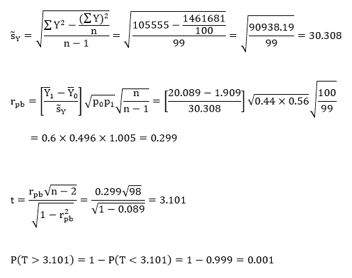
Since our calculated p-value is smaller than our α-level, we reject H0 and conclude that the correlation in the population is significantly greater than zero.
Example in R
x=read.table('clipboard', header=T)
attach(x)
cor.test(favorite, playcount, alternative="greater")
        Pearson's product-moment correlation
data:  favorite and playcount
t = 3.1048, df = 98, p-value = 0.001245
alternative hypothesis: true correlation is greater than 0
95 percent confidence interval:
 0.1407541 1.0000000
sample estimates:
     cor
0.299258
Week 35: The Pearson Product-Moment Correlation Coefficient
Today we’re going to talk about our first measure of association: the Pearson product-moment correlation coefficient!
When Would You Use It?
The Pearson product-moment correlation coefficient is a parametric test used to determine, in the population, if the correlation between values on two variables some value other than zero. More specifically, it is used to determine if there is a significant linear relationship between the two variables.
What Type of Data?
Pearson product-moment correlation coefficient requires interval or ratio data.
Test Assumptions
- The sample has been randomly selected from the population it represents.
- The variables are interval or ratio in nature.
- The two variables have a bivariate normal distribution.
- The assumption of homoscedasticity is met.
- The residuals are independent of one another.
Test Process
Step 1: Formulate the null and alternative hypotheses. The null hypothesis claims that in the population, the correlation between the scores on variable X and variable Y is equal to zero. The alternative hypothesis claims otherwise (that the correlation is less than, greater than, or simply not equal to zero.)
Step 2: Compute the test statistic, a t-value. To do so, the actual correlation coefficient, r, must be calculated first. This calculation is as follows:

To compute the t-statistic, the following equation is used:

Step 3: Obtain the p-value associated with the calculated t-score. The p-value indicates the probability of observing a correlation as extreme or more extreme than the observed sample correlation, under the assumption that the null hypothesis is true.
Step 4: Determine the conclusion. If the p-value is larger than the prespecified α-level, fail to reject the null hypothesis (that is, retain the claim that the correlation in the population is zero). If the p-value is smaller than the prespecified α-level, reject the null hypothesis in favor of the alternative.
Example
I’m going to look at my music data again! I want to see if there is a significant correlation between the length of a song and the number of times I’ve played it. I suspect that I play longer songs less often than shorter ones (I just have a preference for slightly shorter songs, not sure why), so I’m going to guess that there’s a negative correlation. I took a sample of n = 100 songs and let α = 0.05.
H0: ρ = 0
Ha: ρ < 0
Computations:

Since our calculated p-value is larger than our α-level, we fail to reject H0 and conclude that the correlation in the population is not significantly smaller than zero.
Example in R
x=read.table('clipboard', header=T)
attach(x)
cor.test(length, playcount, alternative = "less")
        Pearson's product-moment correlation
data:  length and playcount
t = -1.0232, df = 98, p-value = 0.1544
alternative hypothesis: true correlation is less than 0
95 percent confidence interval:
 -1.00000000  0.06374622
sample estimates:
       cor
-0.102812
Week 34: The Within-Subjects Factorial Analysis of Variance
Today we’re going to look at a test similar to the one we looked at two weeks ago. Specifically, we’re going to look at the within-subjects factorial analysis of variance!
When Would You Use It?
The within-subjects factorial analysis of variance is a parametric test used in cases where a researcher has a factorial design with two* factors, A and B, and has a set of subjects that are measured on each of the levels of all of the factors. The researcher is interested in the following:
- In terms of factor A, in the set of p dependent samples (p ≥ 2), do the factor levels effect the variable of interest across the dependent samples?
- In terms of factor B, in the set of q dependent samples (q ≥ 2), do the factor levels effect the variable of interest across the dependent samples?
- Is there a significant interaction between the two factors?
What Type of Data?
The within-subjects factorial analysis of variance requires interval or ratio data.
Test Assumptions
- Each sample of subjects has been randomly chosen from the population it represents.
- For each sample, the distribution of the data in the underlying population is normal.
- The variances of the k underlying populations are equal (homogeneity of variances).
Test Process
Step 1: Formulate the null and alternative hypotheses. For factor A, the null hypothesis is the claim that the mean of the subjects’ scores across the different levels are equal. The alternative hypothesis claims otherwise. For factor B, the null hypothesis is the claim that the mean of the subjects’ scores across the different levels are equal. The alternative hypothesis claims otherwise. For the interaction, the null hypothesis claims that there is no interaction between factor A and factor B. The alternative claims otherwise.
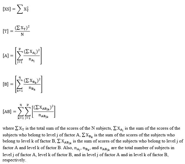
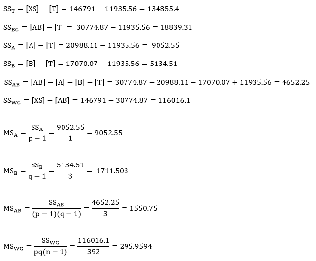
Step 2: Compute the test statistics for the three hypothesis. To do so, we must find SSA, SSB, and SSAB. First, find the following values:

Then, find the SS values as follows:

Then find the MS values:

Finally, compute the three test statistics, F-values, for factor A, factor B, and the interaction.
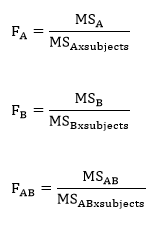
Step 3: Obtain the p-value associated with the calculated F statistics. The p-value indicates the probability of the ratio of the MSA, MSB, or MSAB to MSWG equal to or larger than the observed ratio in the F statistics, under the assumption that the null hypotheses are true.
Step 4: Determine the conclusion. If the p-value is larger than the prespecified α-level (or the calculated F statistic is larger than the critical F value), fail to reject the null hypothesis (that is, retain the claim that the population means are all equal). If the p-value is smaller than the prespecified α-level, reject the null hypothesis in favor of the alternative.
Example
I don’t have a good example of my own for a within-subjects factorial analysis of variance, so I figured I’d use the example from the book! An experimenter employs a two-factor within-subjects design to determine the effects of humidity (factor A, two levels) and temperature (factor B, three levels) on mechanical problem-solving ability.
Here, n = 18 (three subjects across 2 x 3 different conditions) and let α = 0.05.
H0: µlowhumidity = µhighhumidity
Ha: the means are different
H0: µlowtemp = µmodtemp = µhightemp
Ha: at least one pair of means are different
H0: there is no interaction between humidity and temperature
Ha: there is an interaction between humidity and temperature
Computations:


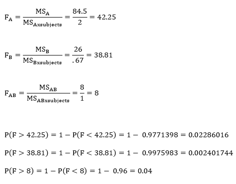
Since all of these p-values are smaller than our α-level of 0.05, we would reject the null hypothesis in all three cases.
Example in R
x=read.table('clipboard', header=T)
attach(x)
fit=aov(score~humidity+temp+humidity:temp)
summary(fit)
*This test can be done with more factors, but for now, let’s just stick with two.
Week 32: The Between-Subjects Factorial Analysis of Variance
Today we’re going back to parametric testing with the between-subjects factorial analysis of variance!
When Would You Use It?
The between-subjects factorial analysis of variance is a parametric test used in cases where a researcher has a factorial design with two* factors, A and B, and is interested in the following:
- In terms of factor A, in the set of p independent samples (p ≥ 2), do at least two of the samples represent populations with different mean values?
- In terms of factor B, in the set of q independent samples (q ≥ 2), do at least two of the samples represent populations with different mean values?
- Is there a significant interaction between the two factors?
What Type of Data?
The between-subjects factorial analysis of variance requires interval or ratio data.
Test Assumptions
- Each sample of subjects has been randomly chosen from the population it represents.
- For each sample, the distribution of the data in the underlying population is normal.
- The variances of the k underlying populations are equal (homogeneity of variances).
Test Process
Step 1: Formulate the null and alternative hypotheses. For factor A, the null hypothesis is the claim mean of the population levels are equal. The alternative hypothesis claims otherwise. For factor B, the null hypothesis is the claim mean of the population levels are equal. The alternative hypothesis claims otherwise. For the interaction, the null hypothesis claims that there is no interaction between factor A and factor B. The alternative claims otherwise.
Step 2: Compute the test statistics for the three hypothesis. To do so, we must find SSA, SSB, and SSAB. First, find the following values:
Then, find the SS values as follows:

Then find the MS values:

Finally, compute the three test statistics, F-values, for factor A, factor B, and the interaction.

Step 3: Obtain the p-value associated with the calculated F statisticS. The p-value indicates the probability of the ratio of the MSA, MSB, or MSAB to MSWG equal to or larger than the observed ratio in the F statistics, under the assumption that the null hypotheses are true.
Step 4: Determine the conclusion. If the p-value is larger than the prespecified α-level (or the calculated F statistic is larger than the critical F value), fail to reject the null hypothesis (that is, retain the claim that the population means are all equal). If the p-value is smaller than the prespecified α-level, reject the null hypothesis in favor of the alternative.
Example
Today’s example looks at my 2015 music data again! I want to see if a) the mean play count is different for those of my songs that are “favorites” (3+ stars) or non-favorites; b) the mean play count is different for any of four genres of interest (alternative, electronic, pop, rock); c) if there is an interaction between these two factors, genre and favorite status. Here, n = 400 and let α = 0.05.
H0: µfavorite = µnofavorite
Ha: the means are different
H0: µalternative = µelectronic = µpop = µrock
Ha: at least one pair of means are different
H0: there is no interaction between favorite status and genre
Ha: there is an interaction between favorite status and genre
Computations:


Since all of these p-values are smaller than our α-level of 0.05, we would reject the null hypothesis in all three cases.
Example in R
x=read.table('clipboard', header=T)
attach(x)
fit=aov(playcount~favorite+genre+favorite:genre)
summary(fit)
                Df Sum Sq Mean Sq F value   Pr(>F)
favorite         1   9053    9053  30.587 5.84e-08 ***
genre            3   4333    1444   4.880 0.002419 **
favorite:genre   3   5454    1818   6.143 0.000433 ***
Residuals      392 116016     296
*This test can be done with more factors, but for now, let’s just stick with two.
Week 31: The Cochran Q Test
Let’s do some more nonparametric testing today with the Cochran Q test!
When Would You Use It?
The Cochran Q test is a nonparametric test used to determine if, in a set of k dependent samples (k ≥ 2), at least two of the samples represent different populations.
What Type of Data?
The Cochran Q test requires categorical or nominal data.
Test Assumptions
- The presentation of the k experimental conditions is random or counterbalanced.
- With matched samples, within each set of matched subjects, each of the subjects should be randomly assigned to one of the k experimental conditions.
Test Process
Step 1: Formulate the null and alternative hypotheses. For the Cochran Q test, we are interested in variables that are dichotomous (let’s say that they have a “yes” and a “no” response). The null hypothesis claims that the proportions of one of the responses is the same across all j experimental conditions. The alternative hypothesis claims otherwise (at least two population proportions are not equal).
Step 2: Compute the test statistic, Q, which is a chi-square value. It is computed as follows:

Step 3: Obtain the p-value associated with the calculated chi-square. The p-value indicates the probability of observing a Q value equal to or larger than the one calculated for the test, under the assumption that the null hypothesis is true.
Step 4: Determine the conclusion. If the p-value is larger than the prespecified α-level, fail to reject the null hypothesis (that is, retain the claim that the proportion of “yes” responses is equal across the k experimental conditions). If the p-value is smaller than the prespecified α-level, reject the null hypothesis in favor of the alternative.
Example
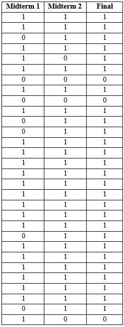
The example for this test comes from a previous semester’s STAT 213 grades. Students took two midterms and a final. I wanted to determine if there was a difference in the proportion of students who passed midterm 1, midterm 2, or the final, in a sample of n = 30. Let α = 0.05.
H0: πmid1 = πmid2 = πfinal
Ha: At least two of the underlying population proportions are not equal.
The following table shows the data for this example. Here, a passing grade is coded as “1” and a failing grade is coded as “0”.
Computations

Since our p-value is larger than our alpha-level, we fail to reject H0 and claim that the proportions for each of the three tests are equal.
Example in R
Since the calculations for this week’s test are quite easy, it’s probably faster to do them by hand than use R!
Ch-Ch-Ch-Chernoff
Want to read about one of the weirdest types of data visualization? Then you want to read about Chernoff faces!
Chernoff faces are as weird as they sound. The idea is to represent different variables as features on a human face. For example, a person’s income could be represented by a Chernoff mouth, with a smile indicating higher incomes and a frown indicating lower incomes. Simultaneously, a person’s health could be represented by Chernoff eyes, with brighter and wider eyes corresponding to good health and tired, listless eyes corresponding to poor health. The more variables there are, the more facial components can be manipulated.
And if you think that sounds like it gets weird, it does:

(source)
The original motivation for Chernoff faces was that humans are basically primed to respond to and interpret faces and face-shaped things. Since we’re so good at interpreting faces, let’s turn data into faces so that we become good at interpreting the data, right?
Well, not really.
One of the main criticisms of Chernoff faces that is mentioned in the above article is that humans respond to faces “as a whole” rather than piece-by-piece. For example, when we look at two faces that differ only in the position of the eyebrows (maybe one has lowered eyebrows and the other has raised eyebrows), we don’t really think of the difference in that way. We think of the faces overall as having different expressions and thus different interpretations. We don’t focus on the eyebrows alone—we focus on the “whole package.”
While this is all well and good for actual faces, it actually makes interpreting changes in variables difficult to understand if those changes are represented by one or two changes on a Chernoff face.
Anyway. It’s actually a really interesting article discussing a really interesting and unique data presentation method. Give it a read!
Week 30: The Friedman Two-Way Analysis of Variance by Ranks
Let’s return to nonparametrics this week with the Friedman two-way analysis of variance by ranks!
When Would You Use It?
The Friedman two-way analysis of variance by ranks is a nonparametric test used to determine if, in a set of k (k ≥ 2) independent samples, at least two of the samples represent populations with different median values.
What Type of Data?
The Friedman two-way analysis of variance by ranks requires ordinal data.
Test Assumptions
- The presentation of the k experimental conditions should be random or counterbalanced.
- If dealing with matched samples, the subjects should be randomly assigned to the k experimental conditions.
Test Process
Step 1: Formulate the null and alternative hypotheses. The null hypothesis claims that the k population medians are equal. The alternative hypothesis claims that at least two of the k population medians are different.
Step 2: Compute the test statistic, a chi-square value. It is computed as follows:

The ranks themselves are obtained by ranking each of the k scores of a subject within that subject. That is, an individual’s scores in each of the k conditions are ranked from highest to lowest (or lowest to highest) for that particular individual. See the example below for more explanation.
Step 3: Obtain the p-value associated with the calculated chi-square statistic. The p-value indicates the probability of observing a chi-square value equal to or larger than the observed chis-square value from the sample under the assumption that the null hypothesis is true. The degrees of freedom for this test are k – 1.
Step 4: Determine the conclusion. If the p-value is larger than the prespecified α-level, fail to reject the null hypothesis (that is, retain the claim that the population medians are equal). If the p-value is smaller than the prespecified α-level, reject the null hypothesis in favor of the alternative.
Example
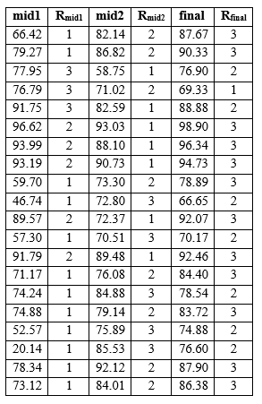
The example I want to look at today is similar to last week’s. The data come from a previous semester’s STAT 213 grades. The class had two midterms and I final. Taking a sample of n = 20 from this class, I wanted to see if the average test grades were all similar across all three tests or if there were some statistically significant differences. Let α = 0.05.
H0: θmidterm1= θmidterm2 = θfinal
Ha: at least one pair of medians are different
The following table shows the midterm and final scores as well as the corresponding within-subject ranks.
Computations:

Here, our computed p-value is smaller than our α-level, which leads us to reject the null hypothesis, which is the claim that the median grade is equal across the three tests.
Example in R
No example in R this week, as this is probably easier to do by hand than using R!
Week 29: The Single-Factor Within-Subjects Analysis of Variance
Let’s change focus a bit this week and look at some ANOVA-related tests for dependent samples. We can start with the single-factor within-subjects analysis of variance!
When Would You Use It?
The single-factor within-subjects analysis of variance is a parametric test used to determine if, in a set of k dependent samples, at least two samples represent populations with different mean values.
What Type of Data?
The single-factor within-subjects analysis of variance requires interval or ratio data.
Test Assumptions
- The sample of subjects has been randomly chosen from the population it represents.
- The distribution of data in the underlying populations for each experimental condition/factor is normal.
- The assumption of sphericity is met.
Test Process
Step 1: Formulate the null and alternative hypotheses. The null hypothesis claims that the k population means are equal. The alternative hypothesis claims that at least two of the k population means are different.
Step 2: Compute the test statistic, an F-value. To do so, calculate the following sums of squares values for between-conditions (SSBC), between-subjects (SSBS), and the residual (SSR):

Then compute the mean squared difference scores for between-subjects (MSBC), between subjects (MSBS), and the residual (MSR):

Finally, compute the F statistic by calculating the ratio:

Step 3: Obtain the p-value associated with the calculated F statistic. The p-value indicates the probability of a ratio of MSBC to MSR equal to or larger than the observed ratio in the F statistic, under the assumption that the null hypothesis is true. Unless you have software, it probably isn’t possible to calculate the exact p-value of your F statistic. Instead, you can use an F table (such as this one) to obtain the critical F value for a prespecified α-level. To use this table, first determine the α-level. Find the degrees of freedom for the numerator (or MSB; the df are explained below) and locate the corresponding column on the table. Then find the degrees of freedom for the denominator (or MSE; the df are explained below) and locate the corresponding set of rows on the table. Find the row specific to your α-level. The value at the intersection of the row and column is your critical F value.
Step 4: Determine the conclusion. If the p-value is larger than the prespecified α-level (or the calculated F statistic is larger than the critical F value), fail to reject the null hypothesis (that is, retain the claim that the population means are all equal). If the p-value is smaller than the prespecified α-level, reject the null hypothesis in favor of the alternative.
Example
The example I want to look at today comes from a previous semester’s STAT 213 grades. The class had two midterms and I final. Taking a sample of n = 30 from this class, I wanted to see if the average test grades were all similar across all three tests or if there were some statistically significant differences. Let α = 0.05.
H0: µmidterm1 = µmidterm2 = µmidterm3
Ha: at least one pair of means are different
Computations:
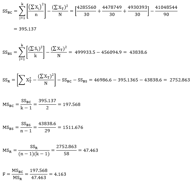
For this case, the critical F value is 3.15. Since the computed F value is larger than the critical F value, we reject H0 and conclude that at least two test grades have population means that are statistically significantly different.
Week 28: The van der Waerden Normal-Scores Test for k Independent Samples
Let’s look at another nonparametric test this week with the van der Waerden normal-scores test for k independent samples!
When Would You Use It?
The van der Waerden normal-scores test for k independent samples is a nonparametric test used to determine if k independend samples are derived from identical population distributions.
What Type of Data?
The van der Waerden normal-scores test for k independent samples requires ordinal data.
Test Assumptions
- Each sample of subjects has been randomly chosen from the population it represents.
- The k samples are independent of one another.
- The dependent variable (the values being ranked) is a continuous random variable.
- The samples’ underlying distributions are identical in shape (but do not necessarily have to be normal).
Test Process
Step 1: Formulate the null and alternative hypotheses. The null hypothesis claims that the k groups are derived from the same population. The alternative hypothesis claims that at least two of the k groups are not derived from the same population.
Step 2: Compute the test statistic, a chi-square value. This value is computed as follows:

Step 3: Obtain the p-value associated with the calculated chi-square statistic. The p-value indicates the probability of observing a chi-square value equal to or larger than the observed chi-sqaure value from the sample under the assumption that the null hypothesis is true. The degrees of freedom for this test are k – 1.
Step 4: Determine the conclusion. If the p-value is larger than the prespecified α-level, fail to reject the null hypothesis (that is, retain the claim that the k groups are derived from the same population). If the p-value is smaller than the prespecified α-level, reject the null hypothesis in favor of the alternative.
Example
The example for this test is the same as the one from last week. Looking at my songs that are rated five stars, I wanted to see if the electronic, alternative, and “other genre” songs were derived from the same population. Here, n = 50 and let α = 0.05.
H0: the k = 3 groups are derived from the same population.
Ha: at least two of the k = 3 groups are not derived from the same population.
The values necessary for this test are displayed in the following tables. The explanations follow.


The first column just contains the raw data values.
The second column contains the ranks. To obtain the ranks of the songs, I did the following steps:
First, I sorted the songs by playcount.
Second, I ranked the songs from 1 to 50 based on their playcount, with 1 corresponding to the song with the highest playcount and 50 corresponding to the song with the lowest playcount. Note that I could have done this the opposite way (1 corresponding to the least-played song and 50 corresponding to the most-played song; the resulting chi-square value would be the same).
Third, I adjusted the ranks for ties. Where there were ties in the playcount, I summed the ranks that were taken by the ties and then divided that value by the number of tied values. I then replaced the original ranks with the newly calculated value.
The third column contains the normal score values for each rank-order. To obtain these values, I did the following:
First, I took each individual rank and divided it by N + 1 = 51. This gave me a proportion that could be conceptualized as the percentile for that score (if multiplied by 100).
Second, I found the standard normal score (z-score) that corresponded to that percentile and input that as the entry for column 3.
Computations
The following three values are the sums of the normal scores for each genre:

And these three values are the average normal scores for each genre:

Here, our computed p-value is greater than our α-level, which leads us to fail to reject the null hypothesis, which is the claim that the three genre groups are derived from the same population.
Example in R
No example in R this week, as this is probably easier to do by hand than using R!
Week 27: The Kruskal-Wallis One-Way Analysis of Variance by Ranks
Back to nonparametrics this week with the Kruskal-Wallis one-way analysis of variance by ranks!
When Would You Use It?
The Kruskal-Wallis one-way analysis of variance by ranks is a nonparametric test used to determine if, in a set of k (k ≥ 2) independent samples, at least two of the samples represent populations with different median values.
What Type of Data?
The Kruskal-Wallis one-way analysis of variance by ranks requires ordinal data.
Test Assumptions
- Each sample of subjects has been randomly chosen from the population it represents.
- The k samples are independent of one another.
- The dependent variable (the values being ranked) is a continuous random variable.
- The distributions of the underlying populations are identical in shape (but do not have to be normal).
Test Process
Step 1: Formulate the null and alternative hypotheses. The null hypothesis claims that the k population medians are equal. The alternative hypothesis claims that at least two of the k population medians are different.
Step 2: Compute the test statistic, a chi-square value (usually denoted as H). H is computed as follows:

Step 3: Obtain the p-value associated with the calculated chi-square H statistic. The p-value indicates the probability of observing an H value equal to or larger than the observed H value from the sample under the assumption that the null hypothesis is true. The degrees of freedom for this test are k – 1.
Step 4: Determine the conclusion. If the p-value is larger than the prespecified α-level, fail to reject the null hypothesis (that is, retain the claim that the population medians are equal). If the p-value is smaller than the prespecified α-level, reject the null hypothesis in favor of the alternative.
Example
The example for this test comes from my music! Looking at my songs that are rated five stars, I wanted to see if there was a difference in the median playcounts for the different genres. Since my Five Star songs are mostly electronic and alternative, I decided to group the rest of the genres into an “other” category so that there are three genre categories total. Here, n = 50 and let α = 0.05.
H0: θelectronic = θalternative = θother
Ha: at least one pair of medians are different
To obtain the ranks of the songs, I did the following steps:
First, I sorted the songs by playcount.
Second, I ranked the songs from 1 to 50 based on their playcount, with 1 corresponding to the song with the highest playcount and 50 corresponding to the song with the lowest playcount. Note that I could have done this the opposite way (1 corresponding to the least-played song and 50 corresponding to the most-played song; the resulting H value would be the same).
Third, I adjusted the ranks for ties. Where there were ties in the playcount, I summed the ranks that were taken by the ties and then divided that value by the number of tied values. I then replaced the original ranks with the newly calculated value.
Finally, I summed the ranks within each of the three genre groups to obtain my Rj values. Here is a table of this final procedure:
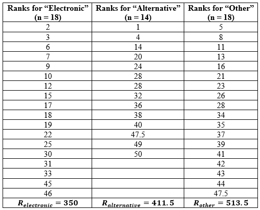
Computations:
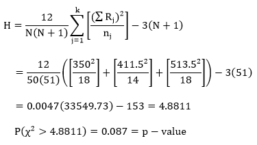
Here, our computed p-value is greater than our α-level, which leads us to fail to reject the null hypothesis, which is the claim that the median playcount is equal across the three genre groups.
Example in R
No example in R this week, as this is probably easier to do by hand than using R!
Week 26: The Single-Factor Between-Subjects Analysis of Variance
We’re back to parametric tests this week with the single-factor between-subjects analysis of variance (ANOVA)!
When Would You Use It?
The single-factor between-subjects ANOVA is a parametric tests used to determine if, in a set of k (k ≥ 2) independent samples, at least two of the samples represent populations with different mean values.
What Type of Data?
The single-factor between-subjects ANOVA requires interval or ratio data.
Test Assumptions
- Each sample of subjects has been randomly chosen from the population it represents.
- For each sample, the distribution of the data in the underlying population is normal.
- The variances of the k underlying populations are equal (homogeneity of variances).
Test Process
Step 1: Formulate the null and alternative hypotheses. The null hypothesis claims that the k population means are equal. The alternative hypothesis claims that at least two of the k population means are different.
Step 2: Compute the test statistic, an F-value. To do so, calculate the following sums of squares values for between-groups (SSB) and within-groups (SSW):
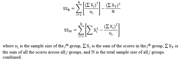
Then compute the mean squared difference scores for between-groups (MSG) and within-groups (MSE):

Finally, compute the F statistic by calculating the ratio:

Step 3: Obtain the p-value associated with the calculated F statistic. The p-value indicates the probability of a ratio of MSB to MSW equal to or larger than the observed ratio in the F statistic, under the assumption that the null hypothesis is true. Unless you have software, it probably isn’t possible to calculate the exact p-value of your F statistic. Instead, you can use an F table (such as this one) to obtain the critical F value for a prespecified α-level. To use this table, first determine the α-level. Find the degrees of freedom for the numerator (or MSB; the df are explained below) and locate the corresponding column on the table. Then find the degrees of freedom for the denominator (or MSE; the df are explained below) and locate the corresponding set of rows on the table. Find the row specific to your α-level. The value at the intersection of the row and column is your critical F value.
Step 4: Determine the conclusion. If the p-value is larger than the prespecified α-level (or the calculated F statistic is larger than the critical F value), fail to reject the null hypothesis (that is, retain the claim that the population means are all equal). If the p-value is smaller than the prespecified α-level, reject the null hypothesis in favor of the alternative.
Example
The example I want to look at today comes from a previous semester’s STAT 217 grades. This particular section of 217 had four labs associated with it. I wanted to determine if the average final grade was different for any one lab compared to the others. Here, n = 109 and let α = 0.05.
H0: µlab1 = µlab2 = µlab3 = µlab4
Ha: at least one pair of means are different
Computations:

For this case, the critical F value, as obtained by the table, is 2.70. Since the computed F value is smaller than the critical F value, we fail to reject H0 and conclude that the average final grade is equal across all four labs.
Example in R

x=read.table('clipboard', header=T)
attach(x)
summary(fit)
             Df Sum Sq Mean Sq F value Pr(>F)
lab           3   1319   439.5   2.036  0.113
Residuals   105  22670   215.9
R will give you the exact p-value of your F statistic; in this case, p-value = 0.113.
Week 25: The McNemar Test
Ready for more nonparametric tests? Today we’re talking about the McNemar test!
When Would You Use It?
The McNemar test is a nonparametric test used to determine if two dependent samples represent two different populations.
What Type of Data?
The McNemar test requires two categorical or nominal data.
Test Assumptions
- The sample of subjects has been randomly chosen from the population it represents.
- Each observation in the contingency table is independent of other observations.
- The scores of the subjects are measured as a dichotomous categorical measure with two mutually exclusive categories.
- The sample size is not “extremely small” (though there is debate over what constitutes an extremely small sample size).
Test Process
Step 1: Formulate the null and alternative hypotheses. For the McNemar test, the data are usually displayed in a contingency table with the following setup:

Here, Response 1 and Response 2 are the two possible outcomes of the first condition. Response A and Response B are the two possible outcomes of the second condition. Cell a represents the number of people in the sample who had both Response 1 and Response A, cell b represents the number of people in the sample who had both Response 1 and Response B, etc.
The null hypothesis of the test claims that in the underlying population represented by the sample, the proportion of observations in cell b is the same as the proportion of observations in cell c. The alternative hypothesis claims otherwise (one population proportion is greater than the other, less than the other, or that the proportions are simply not equal).
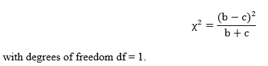
Step 2: Compute the test statistic, a chi-square. It is computed as follows:
Step 3: Obtain the p-value associated with the calculated chi-square. The p-value indicates the probability of a difference in the two cell counts equal to or more extreme than the observed difference between the cell counts, under the assumption that the null hypothesis is true.
Step 4: Determine the conclusion. If the p-value is larger than the prespecified α-level, fail to reject the null hypothesis (that is, retain the claim that the cell proportions for cell b and cell c are equal). If the p-value is smaller than the prespecified α-level, reject the null hypothesis in favor of the alternative.
Example
The example for this test comes from a previous semester’s STAT 217 grades. In the semester in question, the professor offered the students a “bonus test” after their midterms. This was done by allowing the students to essentially re-take the midterm given in class, but doing so on their own time and using all the resources they wanted to. A (small) fraction of the points they would earn on this bonus test would be added to their actual in-class test points.
I wanted to determine if the proportion of students who passed the lab test and failed the bonus test was equal to the proportion of students who failed the lab test but passed the bonus test, using n = 109 students and α = 0.05.
H0: πpass/fail = πfail/pass
Ha: πpass/fail ≠ πfail/pass
The following table shows the breakdown for the four possible outcomes in this case.

Computations:

Since our p-value is smaller than our alpha-level, we reject H0 and claim that the proportions for cells b and c are significantly different.
Example in R
Since the calculations for this week’s test are quite easy, it’s probably faster to do them by hand than use R!

