Week 42: Goodman and Kruskal’s Gamma
Let’s keep going with measures of correlation and talk about Goodman and Kruskal’s gamma today!
When Would You Use It?
Goodman and Kruskal’s gamma is a nonparametric test used to determine, in the population represented by a sample, if the correlation between subjects’ scores on two variables is some value other than zero.
What Type of Data?
Goodman and Kruskal’s gamma requires both variables to be ordinal data.
Test Assumptions
No assumptions listed.
Test Process
Step 1: Formulate the null and alternative hypotheses. The null hypothesis claims that in the population, the correlation between the scores on variable X and variable Y is equal to zero. The alternative hypothesis claims otherwise (that the correlation is less than, greater than, or simply not equal to zero).
Step 2: Compute the test statistic, a z-value. To do so, Goodman and Kruskal’s gamma, G, must be computed first. The following steps must be employed:
- Arrange the data into an ordered r x c contingency table, with r representing the number of levels of the X variable and c representing the number of levels in the Y variable. The first row represents the category that is lowest in magnitude on the X variable and the first column represents the category that is lowest in magnitude on the Y variable. Within each cell of the table is the number of subjects whose categorization on the X and Y variables corresponds to the row and column of the specified cell.
- Calculate nc, the number of pairs of subjects who are concordant with respect to the ordering of their scores on the two variables. This is done as follows, starting at the upper left-hand corner of the table: for each cell, determine the frequency of that cell, then multiply that frequency by the sum of all the frequencies of all cells that fall both below it and to the right of it. The sum of these products is nc.
- Calculate nd, the number of pairs of subjects who are discordant with respect to the ordering of their scores on the two variables. This is done as follows, starting at the upper right-hand corner of the table: for each cell, determine the frequency of that cell, then multiply that frequency by the sum of all the frequencies of all cells that fall both below it and to the left of it. The sum of these products is nd.
- Compute G as follows:
The test statistic itself is calculated as:

Where N is the total number of subjects whose scores are recorded in the contingency table.
Step 3: Obtain the p-value associated with the calculated z-score. The p-value indicates the probability of observing a correlation as extreme or more extreme than the observed sample correlation, under the assumption that the null hypothesis is true.
Step 4: Determine the conclusion. If the p-value is larger than the prespecified α-level, fail to reject the null hypothesis (that is, retain the claim that the correlation in the population is zero). If the p-value is smaller than the prespecified α-level, reject the null hypothesis in favor of the alternative.
Example
Let’s see if there’s a relationship between stars (3, 4, or 5) and what I consider to be my favorite four genres: electronic, pop, alternative, and rock (in that order). Let X be the song’s genre and let Y be the number of stars received by the song. The following is an ordered contingency table of a sample of 400 songs (100 of each genre).

I suspect a positive correlation between ranked favorite genres and stars. Here, n = 400 and let α = 0.05.
H0: γ = 0
Ha: γ > 0
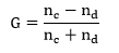
The calculations for nc and nd:
And G and the test statistic:

Since our calculated p-value is smaller than our α-level, we reject H0 and conclude that the correlation in the population is significantly greater than zero.
Week 40: Kendall’s Tau
Let’s do another measure of correlation, shall we? Kendall’s tau!
When Would You Use It?
Kendall’s tau is a nonparametric test used to determine, in the population represented by a sample, if the correlation between subject’s scores on two variables equal to a value other than zero.
What Type of Data?
Kendall’s tau requires both variables to be ordinal data.
Test Assumptions
No assumptions listed.
Test Process
Step 1: Formulate the null and alternative hypotheses. The null hypothesis claims that in the population, the correlation between the ranks of subjects on variable X and variable Y is equal to zero. The alternative hypothesis claims otherwise (that the correlation is less than, greater than, or simply not equal to zero).
Step 2: Compute the test statistic, a z-value. To do so, Kendall’s tau must be computed first. The following steps must be employed:
- Arrange the data by the ranking on the X variable (smallest to largest ranking).
- Begin with the first Y rank corresponding to the first (smallest) X rank. If the Y rank for the smallest X ranking is larger than any Y ranks corresponding to any of the other X ranks, note it with a “D” for discordant. If the Y rank for the smallest X ranking is smaller than any Y ranks corresponding to any other X ranks, note it with a “C” for concordant.
- Once this is done for all comparisons for the first Y rank, move on to the second Y rank and repeat steps 2 and 3 until all ranks are considered.
- For each Y rank, sum the number of Cs and the number of Ds. The sum of all the Cs across all rankings gives you nC, the total number of C entries, and the sum of all the Ds across all rankings gives you nD, the total number of D entries.
Compute Kendall’s tau as follows:

where nC and nD are as defined above and n is the total number of data points in the sample.
The test statistic itself is calculated as:

Step 3: Obtain the p-value associated with the calculated z-score. The p-value indicates the probability of observing a correlation as extreme or more extreme than the observed sample correlation, under the assumption that the null hypothesis is true.
Step 4: Determine the conclusion. If the p-value is larger than the prespecified α-level, fail to reject the null hypothesis (that is, retain the claim that the correlation between the ranks in the population is zero). If the p-value is smaller than the prespecified α-level, reject the null hypothesis in favor of the alternative.
Example
I want to see if there’s a correlation between my ranking of 12 of my songs from 2009 and the ranking of those 12 same songs in 2016. Let X be the ranking in 2009 and Y be the ranking in 2016. Let’s use α = 0.05. I actually have no idea if this will end up a positive or negative correlation, so let’s go with the most general hypotheses:
H0: τ = 0
Ha: τ ≠ 0
The table below shows the rankings of the 12 songs for 2009 and 2016, as well as the method to obtain the sums of Cs and sums of Ds.
nC = 42 and nD = 24
Kendall’s tau and the test statistic:

Since our calculated p-value is larger than our α-level, we fail to reject H0 and conclude that the correlation between the ranks in the population is not significantly different from zero.
Week 39: Spearman’s Rank-Order Correlation Coefficient
Let’s talk about the Spearman’s rank-order correlation coefficient today!
When Would You Use It?
The Spearman’s rank-order correlation coefficient is a nonparametric test used to determine, in the population, if the correlation between values on two variables is some value other than zero. More specifically, it is used to determine if there is a significant linear relationship between the two variables.
What Type of Data?
The Spearman’s rank-order correlation coefficient requires both variables to be ordinal data.
Test Assumptions
No assumptions listed.
Test Process
Step 1: Formulate the null and alternative hypotheses. The null hypothesis claims that in the population, the correlation between the scores on variable X and variable Y is equal to zero. The alternative hypothesis claims otherwise (that the correlation is less than, greater than, or simply not equal to zero).
Step 2: Compute the test statistic, a t value. To do so, Spearman’s rank-order correlation coefficient, rs, must be computed first. The following steps must be employed:
- Rank both variables in order from smallest to largest, assigning a value of “1” to the smallest value for each variable, a “2” for the second-smallest value for each variable, etc.
- For each pair of observations (that is, for each paired value of X and Y, compute di, the difference between the ranked values of Xi and Yi.
- Compute di2, the squared difference of the ranks of Xi and Yi.
- Compute rs as follows:

The test statistic itself is calculated as:
which is a t-value with degrees of freedom n – 2. Here, rs is the Spearman rank-order correlation coefficient and n is the sample size.
Step 3: Obtain the p-value associated with the calculated z-score. The p-value indicates the probability of observing a correlation as extreme or more extreme than the observed sample correlation, under the assumption that the null hypothesis is true.
Step 4: Determine the conclusion. If the p-value is larger than the prespecified α-level, fail to reject the null hypothesis (that is, retain the claim that the correlation in the population is zero). If the p-value is smaller than the prespecified α-level, reject the null hypothesis in favor of the alternative.
Example
Let’s look at a random selection of 10 of my songs and see if there is a significant correlation between the number of stars a song has (its “rating”) and the number of times it has been played (its “playcount”). Let the X variable be the song’s rating and the Y variable be its playcount. I suspect a positive correlation between rating and playcount (or else my rating system is highly flawed!) Here, n = 10 and let α = 0.05.
H0: rs = 0
Ha: rs > 0
The following table shows the raw data and the rankings needed to compute rs.
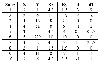
Here Rx and Ry represent the ranks of X and Y, respectively, d represents the difference Rx – Ry, and d2 is the squared differences.
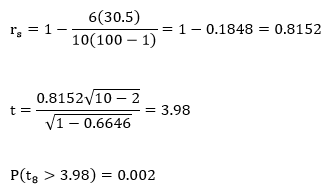
Since our calculated p-value is smaller than our α-level, we reject H0 and conclude that the correlation in the population is significantly greater than zero.
Week 38: The Tetrachoric Correlation Coefficient
Let’s talk about another measure of association today: the tetrachoric correlation coefficient!
When Would You Use It?
The tetrachoric correlation coefficient is a parametric test used to determine, in the population, if the correlation between values on two variables is some value other than zero. More specifically, it is used to determine if there is a significant linear relationship between the two variables.
What Type of Data?
The tetrachoric correlation coefficient requires both variables to be interval or ratio data, but also that both of them have been transformed into dichotomous nominal or ordinal scale variables.
Test Assumptions
- The sample has been randomly selected from the population it represents.
- The underlying distributions for both the variables involved is assumed to be continuous and normal.
Test Process
Step 1: Formulate the null and alternative hypotheses. The null hypothesis claims that in the population, the correlation between the scores on variable X and variable Y is equal to zero. The alternative hypothesis claims otherwise (that the correlation is less than, greater than, or simply not equal to zero).
Step 2: Compute the test statistic, a z-value. To do so, the actual correlation coefficient, rtet, must be calculated first. This calculation requires the information on the variables X and Y to be displayed in a table such as the following:
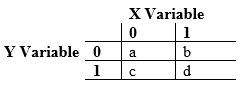
Where “0” and “1” are the coded values of the dichotomous responses for X and Y, and the values a, b, c, and d represent the number of points in the sample that belong to the different combinations of 0 and 1 for the two variables.
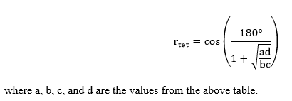
Once the table is constructed, rtet is computed as follows:
To compute the z-statistic, the following equation is used:

To obtain h for each variable, first find the z-value that delineates the point on the normal curve for which the proportion of cases corresponding to the smaller of p0 and p1 falls above that point and the larger of the two proportions p0 and p1 falls below. This table lists the ordinates for specific z-scores.
Step 3: Obtain the p-value associated with the calculated z-score. The p-value indicates the probability of observing a correlation as extreme or more extreme than the observed sample correlation, under the assumption that the null hypothesis is true.
Step 4: Determine the conclusion. If the p-value is larger than the prespecified α-level, fail to reject the null hypothesis (that is, retain the claim that the correlation in the population is zero). If the p-value is smaller than the prespecified α-level, reject the null hypothesis in favor of the alternative.
Example
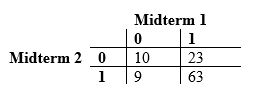
Let’s look at the exam grades for one of the old STAT 213 classes. I want to see if there is a significant correlation between the grades on midterm 1 and midterm 2 as far as whether they got a grade higher than a C+. I will code a grade higher than a C+ as 1 and a grade equal to or lower than a C+ as a 0. Let the X variable be the grade on the first midterm, and the Y variable be the grade on the second midterm. I suspect a negative correlation between X and Y, since a lot of students who did poorly on the first midterm either dropped the class or worked really hard to do well on the second one. Here, n = 105 and let α = 0.05.
H0: ρtet = 0
Ha: ρtet > 0
The following table shows the distribution of the 0’s and 1’s for these two variables:
Computations:
First, let’s find the h values. For midterm 1, p0 = 0.18 and p1 = 0.82. The z-score for which 0.82 of the distribution falls below and 0.21 of the distribution falls above is 0.92. The ordinate, h, of this value is 0.2613 according to the table. For midterm 2, p0 = 0.31 and p1 = 0.69. The z-score for which 0.69 of the distribution falls below and 0.31 of the distribution falls above is 0.5. The ordinate, h, of this value is 0.3521 according to the table. So,

Since our calculated p-value is smaller than our α-level, we reject H0 and conclude that the correlation in the population is significantly greater than zero.
Week 37: The Biserial Correlation Coefficient
Today we’re going to talk about yet another measure of association: the biserial correlation coefficient!
When Would You Use It?
The biserial correlation coefficient is a parametric test used to determine, in the population, if the correlation between values on two variables some value other than zero. More specifically, it is used to determine if there is a significant linear relationship between the two variables.
What Type of Data?
The biserial correlation coefficient requires both variables to be interval or ratio data, but one of these variables to have been transformed into a dichotomous nominal or ordinal scale.
Test Assumptions
- The sample has been randomly selected from the population it represents.
- The underlying distributions for both the variables involved is assumed to be continuous and normal.
Test Process
Step 1: Formulate the null and alternative hypotheses. The null hypothesis claims that in the population, the correlation between the scores on variable X and variable Y is equal to zero. The alternative hypothesis claims otherwise (that the correlation is less than, greater than, or simply not equal to zero).
Step 2: Compute the test statistic, a z-value. To do so, the actual correlation coefficient, rb, must be calculated first. This calculation is as follows:

The value h represents the ordinate of the point in the standard normal distribution that divides the proportions p0 and p1. To obtain h, first find the z-value that delineates the point on the normal curve for which the proportion of cases corresponding to the smaller of p0 and p1 falls above that point and the larger of the two proportions p0 and p1 falls below. This table lists the ordinates for specific z-scores.
To compute the z-statistic, the following equation is used:

Step 3: Obtain the p-value associated with the calculated z-score. The p-value indicates the probability of observing a correlation as extreme or more extreme than the observed sample correlation, under the assumption that the null hypothesis is true.
Step 4: Determine the conclusion. If the p-value is larger than the prespecified α-level, fail to reject the null hypothesis (that is, retain the claim that the correlation in the population is zero). If the p-value is smaller than the prespecified α-level, reject the null hypothesis in favor of the alternative.
Example
Let’s look at the exam grades for one of the old STAT 213 classes. I want to see if there is a significant correlation between the average grade of students’ two midterm tests and whether or not they got a grade higher than a C+ on the final. I will code a grade higher than a C+ as 1 and a grade equal to or lower than a C+ as a 0. I suspect a positive correlation. Here, n = 107 and let α = 0.05.
H0: ρb = 0
Ha: ρb > 0
Computations:
First, let’s find h. In the sample, p0 = 0.28 and p1 = 0.72. The z-score for which 0.72 of the distribution falls below and 0.28 of the distribution falls above is 0.58. The ordinate, h, of this value is 0.3372 according to the table. So,

Since our calculated p-value is larger than our α-level, we fail to reject H0 and conclude that the correlation in the population is not significantly greater than zero.
Week 36: The Point-Biserial Correlation Coefficient
Today we’re going to talk about another measure of association: the point-biserial correlation coefficient!
When Would You Use It?
The point-biserial correlation coefficient is a parametric test used to determine, in the population, if the correlation between values on two variables some value other than zero. More specifically, it is used to determine if there is a significant linear relationship between the two variables.
What Type of Data?
The point-biserial correlation coefficient requires one variable to be expressed as interval or ratio data and the other variable to be represented by a dichotomous nominal or categorical scale. The point-biserial correlation coefficient is a special case of the Pearson product-moment correlation coefficient requires interval or ratio data.
Test Assumptions
- The sample has been randomly selected from the population it represents.
- The dichonomous variable is not based on an underlying continuous interval or ratio distribution.
Test Process
Step 1: Formulate the null and alternative hypotheses. The null hypothesis claims that in the population, the correlation between the scores on variable X and variable Y is equal to zero. The alternative hypothesis claims otherwise (that the correlation is less than, greater than, or simply not equal to zero.)
Step 2: Compute the test statistic, a t-value. To do so, the actual correlation coefficient, rpb, must be calculated first. This calculation is as follows:
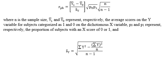
To compute the t-statistic, the following equation is used:
Step 3: Obtain the p-value associated with the calculated t-score. The p-value indicates the probability of observing a correlation as extreme or more extreme than the observed sample correlation, under the assumption that the null hypothesis is true.
Step 4: Determine the conclusion. If the p-value is larger than the prespecified α-level, fail to reject the null hypothesis (that is, retain the claim that the correlation in the population is zero). If the p-value is smaller than the prespecified α-level, reject the null hypothesis in favor of the alternative.
Example
Let’s look at my music data again! I want to see if there is a significant correlation between the number of times I’ve played a song and whether or not it is a “favorite” (i.e., has 3+ stars). I suspect, of course, that I play my favorite songs more often than my non-favorite ones. If I code “favorite” as 1 and “non-favorite” as 0, then I will expect a positive correlation. I took a sample of n = 100 songs and let α = 0.05.
H0: ρpb = 0
Ha: ρpb > 0
Computations:

Since our calculated p-value is smaller than our α-level, we reject H0 and conclude that the correlation in the population is significantly greater than zero.
Example in R
x=read.table('clipboard', header=T)
attach(x)
cor.test(favorite, playcount, alternative="greater")
        Pearson's product-moment correlation
data:  favorite and playcount
t = 3.1048, df = 98, p-value = 0.001245
alternative hypothesis: true correlation is greater than 0
95 percent confidence interval:
 0.1407541 1.0000000
sample estimates:
     cor
0.299258
Week 35: The Pearson Product-Moment Correlation Coefficient
Today we’re going to talk about our first measure of association: the Pearson product-moment correlation coefficient!
When Would You Use It?
The Pearson product-moment correlation coefficient is a parametric test used to determine, in the population, if the correlation between values on two variables some value other than zero. More specifically, it is used to determine if there is a significant linear relationship between the two variables.
What Type of Data?
Pearson product-moment correlation coefficient requires interval or ratio data.
Test Assumptions
- The sample has been randomly selected from the population it represents.
- The variables are interval or ratio in nature.
- The two variables have a bivariate normal distribution.
- The assumption of homoscedasticity is met.
- The residuals are independent of one another.
Test Process
Step 1: Formulate the null and alternative hypotheses. The null hypothesis claims that in the population, the correlation between the scores on variable X and variable Y is equal to zero. The alternative hypothesis claims otherwise (that the correlation is less than, greater than, or simply not equal to zero.)
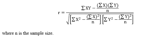
Step 2: Compute the test statistic, a t-value. To do so, the actual correlation coefficient, r, must be calculated first. This calculation is as follows:
To compute the t-statistic, the following equation is used:
Step 3: Obtain the p-value associated with the calculated t-score. The p-value indicates the probability of observing a correlation as extreme or more extreme than the observed sample correlation, under the assumption that the null hypothesis is true.
Step 4: Determine the conclusion. If the p-value is larger than the prespecified α-level, fail to reject the null hypothesis (that is, retain the claim that the correlation in the population is zero). If the p-value is smaller than the prespecified α-level, reject the null hypothesis in favor of the alternative.
Example
I’m going to look at my music data again! I want to see if there is a significant correlation between the length of a song and the number of times I’ve played it. I suspect that I play longer songs less often than shorter ones (I just have a preference for slightly shorter songs, not sure why), so I’m going to guess that there’s a negative correlation. I took a sample of n = 100 songs and let α = 0.05.
H0: ρ = 0
Ha: ρ < 0
Computations:
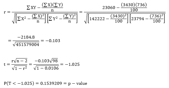
Since our calculated p-value is larger than our α-level, we fail to reject H0 and conclude that the correlation in the population is not significantly smaller than zero.
Example in R
x=read.table('clipboard', header=T)
attach(x)
cor.test(length, playcount, alternative = "less")
        Pearson's product-moment correlation
data:  length and playcount
t = -1.0232, df = 98, p-value = 0.1544
alternative hypothesis: true correlation is less than 0
95 percent confidence interval:
 -1.00000000  0.06374622
sample estimates:
       cor
-0.102812
Week 34: The Within-Subjects Factorial Analysis of Variance
Today we’re going to look at a test similar to the one we looked at two weeks ago. Specifically, we’re going to look at the within-subjects factorial analysis of variance!
When Would You Use It?
The within-subjects factorial analysis of variance is a parametric test used in cases where a researcher has a factorial design with two* factors, A and B, and has a set of subjects that are measured on each of the levels of all of the factors. The researcher is interested in the following:
- In terms of factor A, in the set of p dependent samples (p ≥ 2), do the factor levels effect the variable of interest across the dependent samples?
- In terms of factor B, in the set of q dependent samples (q ≥ 2), do the factor levels effect the variable of interest across the dependent samples?
- Is there a significant interaction between the two factors?
What Type of Data?
The within-subjects factorial analysis of variance requires interval or ratio data.
Test Assumptions
- Each sample of subjects has been randomly chosen from the population it represents.
- For each sample, the distribution of the data in the underlying population is normal.
- The variances of the k underlying populations are equal (homogeneity of variances).
Test Process
Step 1: Formulate the null and alternative hypotheses. For factor A, the null hypothesis is the claim that the mean of the subjects’ scores across the different levels are equal. The alternative hypothesis claims otherwise. For factor B, the null hypothesis is the claim that the mean of the subjects’ scores across the different levels are equal. The alternative hypothesis claims otherwise. For the interaction, the null hypothesis claims that there is no interaction between factor A and factor B. The alternative claims otherwise.
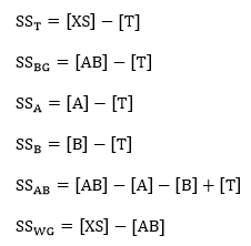
Step 2: Compute the test statistics for the three hypothesis. To do so, we must find SSA, SSB, and SSAB. First, find the following values:
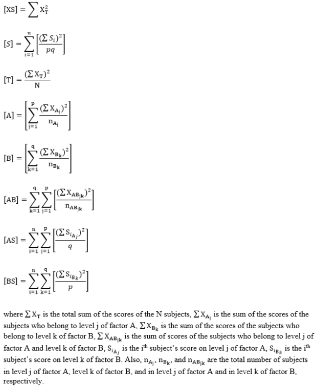
Then, find the SS values as follows:

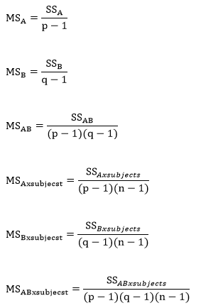
Then find the MS values:
Finally, compute the three test statistics, F-values, for factor A, factor B, and the interaction.

Step 3: Obtain the p-value associated with the calculated F statistics. The p-value indicates the probability of the ratio of the MSA, MSB, or MSAB to MSWG equal to or larger than the observed ratio in the F statistics, under the assumption that the null hypotheses are true.
Step 4: Determine the conclusion. If the p-value is larger than the prespecified α-level (or the calculated F statistic is larger than the critical F value), fail to reject the null hypothesis (that is, retain the claim that the population means are all equal). If the p-value is smaller than the prespecified α-level, reject the null hypothesis in favor of the alternative.
Example
I don’t have a good example of my own for a within-subjects factorial analysis of variance, so I figured I’d use the example from the book! An experimenter employs a two-factor within-subjects design to determine the effects of humidity (factor A, two levels) and temperature (factor B, three levels) on mechanical problem-solving ability.
Here, n = 18 (three subjects across 2 x 3 different conditions) and let α = 0.05.
H0: µlowhumidity = µhighhumidity
Ha: the means are different
H0: µlowtemp = µmodtemp = µhightemp
Ha: at least one pair of means are different
H0: there is no interaction between humidity and temperature
Ha: there is an interaction between humidity and temperature
Computations:


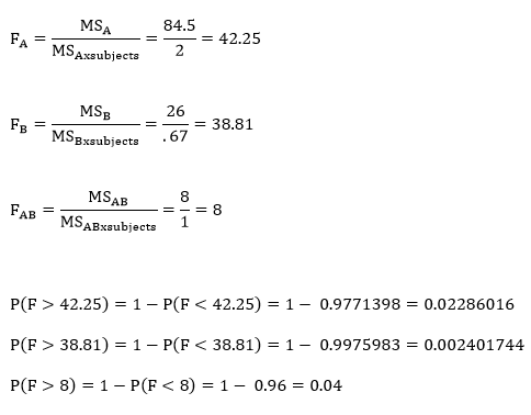
Since all of these p-values are smaller than our α-level of 0.05, we would reject the null hypothesis in all three cases.
Example in R
x=read.table('clipboard', header=T)
attach(x)
fit=aov(score~humidity+temp+humidity:temp)
summary(fit)
*This test can be done with more factors, but for now, let’s just stick with two.
Week 32: The Between-Subjects Factorial Analysis of Variance
Today we’re going back to parametric testing with the between-subjects factorial analysis of variance!
When Would You Use It?
The between-subjects factorial analysis of variance is a parametric test used in cases where a researcher has a factorial design with two* factors, A and B, and is interested in the following:
- In terms of factor A, in the set of p independent samples (p ≥ 2), do at least two of the samples represent populations with different mean values?
- In terms of factor B, in the set of q independent samples (q ≥ 2), do at least two of the samples represent populations with different mean values?
- Is there a significant interaction between the two factors?
What Type of Data?
The between-subjects factorial analysis of variance requires interval or ratio data.
Test Assumptions
- Each sample of subjects has been randomly chosen from the population it represents.
- For each sample, the distribution of the data in the underlying population is normal.
- The variances of the k underlying populations are equal (homogeneity of variances).
Test Process
Step 1: Formulate the null and alternative hypotheses. For factor A, the null hypothesis is the claim mean of the population levels are equal. The alternative hypothesis claims otherwise. For factor B, the null hypothesis is the claim mean of the population levels are equal. The alternative hypothesis claims otherwise. For the interaction, the null hypothesis claims that there is no interaction between factor A and factor B. The alternative claims otherwise.
Step 2: Compute the test statistics for the three hypothesis. To do so, we must find SSA, SSB, and SSAB. First, find the following values:

Then, find the SS values as follows:
Then find the MS values:

Finally, compute the three test statistics, F-values, for factor A, factor B, and the interaction.

Step 3: Obtain the p-value associated with the calculated F statisticS. The p-value indicates the probability of the ratio of the MSA, MSB, or MSAB to MSWG equal to or larger than the observed ratio in the F statistics, under the assumption that the null hypotheses are true.
Step 4: Determine the conclusion. If the p-value is larger than the prespecified α-level (or the calculated F statistic is larger than the critical F value), fail to reject the null hypothesis (that is, retain the claim that the population means are all equal). If the p-value is smaller than the prespecified α-level, reject the null hypothesis in favor of the alternative.
Example
Today’s example looks at my 2015 music data again! I want to see if a) the mean play count is different for those of my songs that are “favorites” (3+ stars) or non-favorites; b) the mean play count is different for any of four genres of interest (alternative, electronic, pop, rock); c) if there is an interaction between these two factors, genre and favorite status. Here, n = 400 and let α = 0.05.
H0: µfavorite = µnofavorite
Ha: the means are different
H0: µalternative = µelectronic = µpop = µrock
Ha: at least one pair of means are different
H0: there is no interaction between favorite status and genre
Ha: there is an interaction between favorite status and genre
Computations:

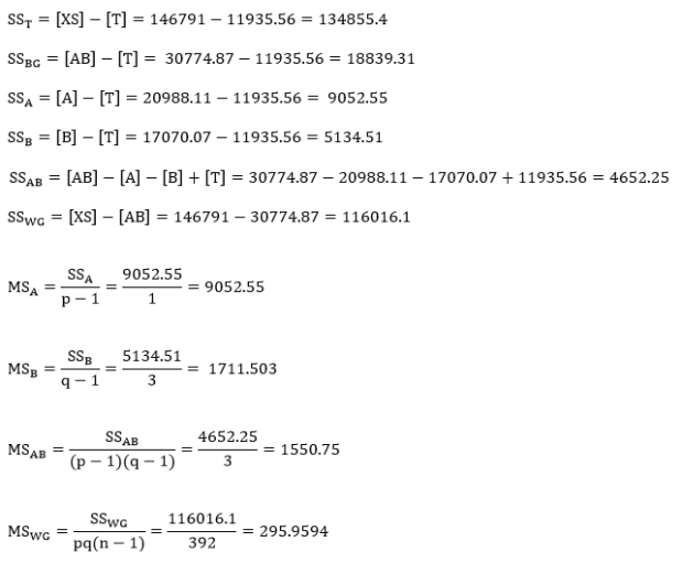

Since all of these p-values are smaller than our α-level of 0.05, we would reject the null hypothesis in all three cases.
Example in R
x=read.table('clipboard', header=T)
attach(x)
fit=aov(playcount~favorite+genre+favorite:genre)
summary(fit)
                Df Sum Sq Mean Sq F value   Pr(>F)
favorite         1   9053    9053  30.587 5.84e-08 ***
genre            3   4333    1444   4.880 0.002419 **
favorite:genre   3   5454    1818   6.143 0.000433 ***
Residuals      392 116016     296
*This test can be done with more factors, but for now, let’s just stick with two.
Week 31: The Cochran Q Test
Let’s do some more nonparametric testing today with the Cochran Q test!
When Would You Use It?
The Cochran Q test is a nonparametric test used to determine if, in a set of k dependent samples (k ≥ 2), at least two of the samples represent different populations.
What Type of Data?
The Cochran Q test requires categorical or nominal data.
Test Assumptions
- The presentation of the k experimental conditions is random or counterbalanced.
- With matched samples, within each set of matched subjects, each of the subjects should be randomly assigned to one of the k experimental conditions.
Test Process
Step 1: Formulate the null and alternative hypotheses. For the Cochran Q test, we are interested in variables that are dichotomous (let’s say that they have a “yes” and a “no” response). The null hypothesis claims that the proportions of one of the responses is the same across all j experimental conditions. The alternative hypothesis claims otherwise (at least two population proportions are not equal).
Step 2: Compute the test statistic, Q, which is a chi-square value. It is computed as follows:

Step 3: Obtain the p-value associated with the calculated chi-square. The p-value indicates the probability of observing a Q value equal to or larger than the one calculated for the test, under the assumption that the null hypothesis is true.
Step 4: Determine the conclusion. If the p-value is larger than the prespecified α-level, fail to reject the null hypothesis (that is, retain the claim that the proportion of “yes” responses is equal across the k experimental conditions). If the p-value is smaller than the prespecified α-level, reject the null hypothesis in favor of the alternative.
Example
The example for this test comes from a previous semester’s STAT 213 grades. Students took two midterms and a final. I wanted to determine if there was a difference in the proportion of students who passed midterm 1, midterm 2, or the final, in a sample of n = 30. Let α = 0.05.
H0: πmid1 = πmid2 = πfinal
Ha: At least two of the underlying population proportions are not equal.
The following table shows the data for this example. Here, a passing grade is coded as “1” and a failing grade is coded as “0”.

Computations
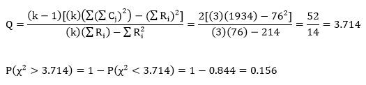
Since our p-value is larger than our alpha-level, we fail to reject H0 and claim that the proportions for each of the three tests are equal.
Example in R
Since the calculations for this week’s test are quite easy, it’s probably faster to do them by hand than use R!
Week 30: The Friedman Two-Way Analysis of Variance by Ranks
Let’s return to nonparametrics this week with the Friedman two-way analysis of variance by ranks!
When Would You Use It?
The Friedman two-way analysis of variance by ranks is a nonparametric test used to determine if, in a set of k (k ≥ 2) independent samples, at least two of the samples represent populations with different median values.
What Type of Data?
The Friedman two-way analysis of variance by ranks requires ordinal data.
Test Assumptions
- The presentation of the k experimental conditions should be random or counterbalanced.
- If dealing with matched samples, the subjects should be randomly assigned to the k experimental conditions.
Test Process
Step 1: Formulate the null and alternative hypotheses. The null hypothesis claims that the k population medians are equal. The alternative hypothesis claims that at least two of the k population medians are different.
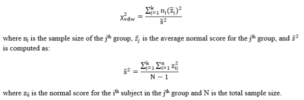
Step 2: Compute the test statistic, a chi-square value. It is computed as follows:

The ranks themselves are obtained by ranking each of the k scores of a subject within that subject. That is, an individual’s scores in each of the k conditions are ranked from highest to lowest (or lowest to highest) for that particular individual. See the example below for more explanation.
Step 3: Obtain the p-value associated with the calculated chi-square statistic. The p-value indicates the probability of observing a chi-square value equal to or larger than the observed chis-square value from the sample under the assumption that the null hypothesis is true. The degrees of freedom for this test are k – 1.
Step 4: Determine the conclusion. If the p-value is larger than the prespecified α-level, fail to reject the null hypothesis (that is, retain the claim that the population medians are equal). If the p-value is smaller than the prespecified α-level, reject the null hypothesis in favor of the alternative.
Example
The example I want to look at today is similar to last week’s. The data come from a previous semester’s STAT 213 grades. The class had two midterms and I final. Taking a sample of n = 20 from this class, I wanted to see if the average test grades were all similar across all three tests or if there were some statistically significant differences. Let α = 0.05.
H0: θmidterm1= θmidterm2 = θfinal
Ha: at least one pair of medians are different
The following table shows the midterm and final scores as well as the corresponding within-subject ranks.
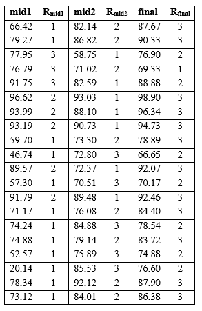
Computations:

Here, our computed p-value is smaller than our α-level, which leads us to reject the null hypothesis, which is the claim that the median grade is equal across the three tests.
Example in R
No example in R this week, as this is probably easier to do by hand than using R!
Week 29: The Single-Factor Within-Subjects Analysis of Variance
Let’s change focus a bit this week and look at some ANOVA-related tests for dependent samples. We can start with the single-factor within-subjects analysis of variance!
When Would You Use It?
The single-factor within-subjects analysis of variance is a parametric test used to determine if, in a set of k dependent samples, at least two samples represent populations with different mean values.
What Type of Data?
The single-factor within-subjects analysis of variance requires interval or ratio data.
Test Assumptions
- The sample of subjects has been randomly chosen from the population it represents.
- The distribution of data in the underlying populations for each experimental condition/factor is normal.
- The assumption of sphericity is met.
Test Process
Step 1: Formulate the null and alternative hypotheses. The null hypothesis claims that the k population means are equal. The alternative hypothesis claims that at least two of the k population means are different.
Step 2: Compute the test statistic, an F-value. To do so, calculate the following sums of squares values for between-conditions (SSBC), between-subjects (SSBS), and the residual (SSR):

Then compute the mean squared difference scores for between-subjects (MSBC), between subjects (MSBS), and the residual (MSR):

Finally, compute the F statistic by calculating the ratio:

Step 3: Obtain the p-value associated with the calculated F statistic. The p-value indicates the probability of a ratio of MSBC to MSR equal to or larger than the observed ratio in the F statistic, under the assumption that the null hypothesis is true. Unless you have software, it probably isn’t possible to calculate the exact p-value of your F statistic. Instead, you can use an F table (such as this one) to obtain the critical F value for a prespecified α-level. To use this table, first determine the α-level. Find the degrees of freedom for the numerator (or MSB; the df are explained below) and locate the corresponding column on the table. Then find the degrees of freedom for the denominator (or MSE; the df are explained below) and locate the corresponding set of rows on the table. Find the row specific to your α-level. The value at the intersection of the row and column is your critical F value.
Step 4: Determine the conclusion. If the p-value is larger than the prespecified α-level (or the calculated F statistic is larger than the critical F value), fail to reject the null hypothesis (that is, retain the claim that the population means are all equal). If the p-value is smaller than the prespecified α-level, reject the null hypothesis in favor of the alternative.
Example
The example I want to look at today comes from a previous semester’s STAT 213 grades. The class had two midterms and I final. Taking a sample of n = 30 from this class, I wanted to see if the average test grades were all similar across all three tests or if there were some statistically significant differences. Let α = 0.05.
H0: µmidterm1 = µmidterm2 = µmidterm3
Ha: at least one pair of means are different
Computations:

For this case, the critical F value is 3.15. Since the computed F value is larger than the critical F value, we reject H0 and conclude that at least two test grades have population means that are statistically significantly different.
Week 28: The van der Waerden Normal-Scores Test for k Independent Samples
Let’s look at another nonparametric test this week with the van der Waerden normal-scores test for k independent samples!
When Would You Use It?
The van der Waerden normal-scores test for k independent samples is a nonparametric test used to determine if k independend samples are derived from identical population distributions.
What Type of Data?
The van der Waerden normal-scores test for k independent samples requires ordinal data.
Test Assumptions
- Each sample of subjects has been randomly chosen from the population it represents.
- The k samples are independent of one another.
- The dependent variable (the values being ranked) is a continuous random variable.
- The samples’ underlying distributions are identical in shape (but do not necessarily have to be normal).
Test Process
Step 1: Formulate the null and alternative hypotheses. The null hypothesis claims that the k groups are derived from the same population. The alternative hypothesis claims that at least two of the k groups are not derived from the same population.
Step 2: Compute the test statistic, a chi-square value. This value is computed as follows:
Step 3: Obtain the p-value associated with the calculated chi-square statistic. The p-value indicates the probability of observing a chi-square value equal to or larger than the observed chi-sqaure value from the sample under the assumption that the null hypothesis is true. The degrees of freedom for this test are k – 1.
Step 4: Determine the conclusion. If the p-value is larger than the prespecified α-level, fail to reject the null hypothesis (that is, retain the claim that the k groups are derived from the same population). If the p-value is smaller than the prespecified α-level, reject the null hypothesis in favor of the alternative.
Example
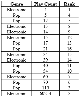
The example for this test is the same as the one from last week. Looking at my songs that are rated five stars, I wanted to see if the electronic, alternative, and “other genre” songs were derived from the same population. Here, n = 50 and let α = 0.05.
H0: the k = 3 groups are derived from the same population.
Ha: at least two of the k = 3 groups are not derived from the same population.
The values necessary for this test are displayed in the following tables. The explanations follow.


The first column just contains the raw data values.
The second column contains the ranks. To obtain the ranks of the songs, I did the following steps:
First, I sorted the songs by playcount.
Second, I ranked the songs from 1 to 50 based on their playcount, with 1 corresponding to the song with the highest playcount and 50 corresponding to the song with the lowest playcount. Note that I could have done this the opposite way (1 corresponding to the least-played song and 50 corresponding to the most-played song; the resulting chi-square value would be the same).
Third, I adjusted the ranks for ties. Where there were ties in the playcount, I summed the ranks that were taken by the ties and then divided that value by the number of tied values. I then replaced the original ranks with the newly calculated value.
The third column contains the normal score values for each rank-order. To obtain these values, I did the following:
First, I took each individual rank and divided it by N + 1 = 51. This gave me a proportion that could be conceptualized as the percentile for that score (if multiplied by 100).
Second, I found the standard normal score (z-score) that corresponded to that percentile and input that as the entry for column 3.
Computations
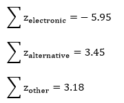
The following three values are the sums of the normal scores for each genre:
And these three values are the average normal scores for each genre:
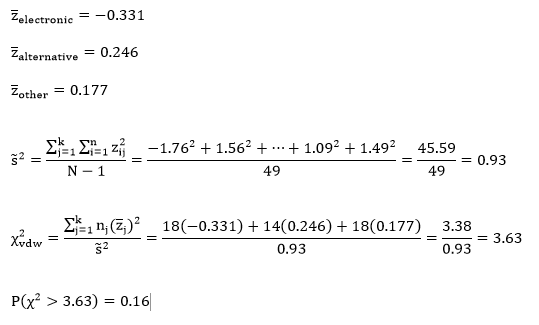
Here, our computed p-value is greater than our α-level, which leads us to fail to reject the null hypothesis, which is the claim that the three genre groups are derived from the same population.
Example in R
No example in R this week, as this is probably easier to do by hand than using R!
Week 27: The Kruskal-Wallis One-Way Analysis of Variance by Ranks
Back to nonparametrics this week with the Kruskal-Wallis one-way analysis of variance by ranks!
When Would You Use It?
The Kruskal-Wallis one-way analysis of variance by ranks is a nonparametric test used to determine if, in a set of k (k ≥ 2) independent samples, at least two of the samples represent populations with different median values.
What Type of Data?
The Kruskal-Wallis one-way analysis of variance by ranks requires ordinal data.
Test Assumptions
- Each sample of subjects has been randomly chosen from the population it represents.
- The k samples are independent of one another.
- The dependent variable (the values being ranked) is a continuous random variable.
- The distributions of the underlying populations are identical in shape (but do not have to be normal).
Test Process
Step 1: Formulate the null and alternative hypotheses. The null hypothesis claims that the k population medians are equal. The alternative hypothesis claims that at least two of the k population medians are different.
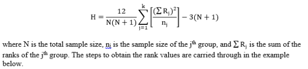
Step 2: Compute the test statistic, a chi-square value (usually denoted as H). H is computed as follows:
Step 3: Obtain the p-value associated with the calculated chi-square H statistic. The p-value indicates the probability of observing an H value equal to or larger than the observed H value from the sample under the assumption that the null hypothesis is true. The degrees of freedom for this test are k – 1.
Step 4: Determine the conclusion. If the p-value is larger than the prespecified α-level, fail to reject the null hypothesis (that is, retain the claim that the population medians are equal). If the p-value is smaller than the prespecified α-level, reject the null hypothesis in favor of the alternative.
Example
The example for this test comes from my music! Looking at my songs that are rated five stars, I wanted to see if there was a difference in the median playcounts for the different genres. Since my Five Star songs are mostly electronic and alternative, I decided to group the rest of the genres into an “other” category so that there are three genre categories total. Here, n = 50 and let α = 0.05.
H0: θelectronic = θalternative = θother
Ha: at least one pair of medians are different
To obtain the ranks of the songs, I did the following steps:
First, I sorted the songs by playcount.
Second, I ranked the songs from 1 to 50 based on their playcount, with 1 corresponding to the song with the highest playcount and 50 corresponding to the song with the lowest playcount. Note that I could have done this the opposite way (1 corresponding to the least-played song and 50 corresponding to the most-played song; the resulting H value would be the same).
Third, I adjusted the ranks for ties. Where there were ties in the playcount, I summed the ranks that were taken by the ties and then divided that value by the number of tied values. I then replaced the original ranks with the newly calculated value.
Finally, I summed the ranks within each of the three genre groups to obtain my Rj values. Here is a table of this final procedure:

Computations:
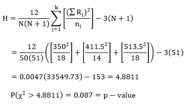
Here, our computed p-value is greater than our α-level, which leads us to fail to reject the null hypothesis, which is the claim that the median playcount is equal across the three genre groups.
Example in R
No example in R this week, as this is probably easier to do by hand than using R!
Week 26: The Single-Factor Between-Subjects Analysis of Variance
We’re back to parametric tests this week with the single-factor between-subjects analysis of variance (ANOVA)!
When Would You Use It?
The single-factor between-subjects ANOVA is a parametric tests used to determine if, in a set of k (k ≥ 2) independent samples, at least two of the samples represent populations with different mean values.
What Type of Data?
The single-factor between-subjects ANOVA requires interval or ratio data.
Test Assumptions
- Each sample of subjects has been randomly chosen from the population it represents.
- For each sample, the distribution of the data in the underlying population is normal.
- The variances of the k underlying populations are equal (homogeneity of variances).
Test Process
Step 1: Formulate the null and alternative hypotheses. The null hypothesis claims that the k population means are equal. The alternative hypothesis claims that at least two of the k population means are different.
Step 2: Compute the test statistic, an F-value. To do so, calculate the following sums of squares values for between-groups (SSB) and within-groups (SSW):
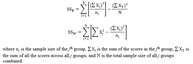
Then compute the mean squared difference scores for between-groups (MSG) and within-groups (MSE):

Finally, compute the F statistic by calculating the ratio:

Step 3: Obtain the p-value associated with the calculated F statistic. The p-value indicates the probability of a ratio of MSB to MSW equal to or larger than the observed ratio in the F statistic, under the assumption that the null hypothesis is true. Unless you have software, it probably isn’t possible to calculate the exact p-value of your F statistic. Instead, you can use an F table (such as this one) to obtain the critical F value for a prespecified α-level. To use this table, first determine the α-level. Find the degrees of freedom for the numerator (or MSB; the df are explained below) and locate the corresponding column on the table. Then find the degrees of freedom for the denominator (or MSE; the df are explained below) and locate the corresponding set of rows on the table. Find the row specific to your α-level. The value at the intersection of the row and column is your critical F value.
Step 4: Determine the conclusion. If the p-value is larger than the prespecified α-level (or the calculated F statistic is larger than the critical F value), fail to reject the null hypothesis (that is, retain the claim that the population means are all equal). If the p-value is smaller than the prespecified α-level, reject the null hypothesis in favor of the alternative.
Example
The example I want to look at today comes from a previous semester’s STAT 217 grades. This particular section of 217 had four labs associated with it. I wanted to determine if the average final grade was different for any one lab compared to the others. Here, n = 109 and let α = 0.05.
H0: µlab1 = µlab2 = µlab3 = µlab4
Ha: at least one pair of means are different
Computations:

For this case, the critical F value, as obtained by the table, is 2.70. Since the computed F value is smaller than the critical F value, we fail to reject H0 and conclude that the average final grade is equal across all four labs.
Example in R

x=read.table('clipboard', header=T)
attach(x)
summary(fit)
             Df Sum Sq Mean Sq F value Pr(>F)
lab           3   1319   439.5   2.036  0.113
Residuals   105  22670   215.9
R will give you the exact p-value of your F statistic; in this case, p-value = 0.113.
Week 25: The McNemar Test
Ready for more nonparametric tests? Today we’re talking about the McNemar test!
When Would You Use It?
The McNemar test is a nonparametric test used to determine if two dependent samples represent two different populations.
What Type of Data?
The McNemar test requires two categorical or nominal data.
Test Assumptions
- The sample of subjects has been randomly chosen from the population it represents.
- Each observation in the contingency table is independent of other observations.
- The scores of the subjects are measured as a dichotomous categorical measure with two mutually exclusive categories.
- The sample size is not “extremely small” (though there is debate over what constitutes an extremely small sample size).
Test Process
Step 1: Formulate the null and alternative hypotheses. For the McNemar test, the data are usually displayed in a contingency table with the following setup:

Here, Response 1 and Response 2 are the two possible outcomes of the first condition. Response A and Response B are the two possible outcomes of the second condition. Cell a represents the number of people in the sample who had both Response 1 and Response A, cell b represents the number of people in the sample who had both Response 1 and Response B, etc.
The null hypothesis of the test claims that in the underlying population represented by the sample, the proportion of observations in cell b is the same as the proportion of observations in cell c. The alternative hypothesis claims otherwise (one population proportion is greater than the other, less than the other, or that the proportions are simply not equal).
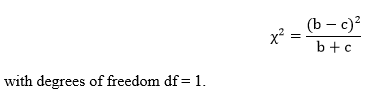
Step 2: Compute the test statistic, a chi-square. It is computed as follows:
Step 3: Obtain the p-value associated with the calculated chi-square. The p-value indicates the probability of a difference in the two cell counts equal to or more extreme than the observed difference between the cell counts, under the assumption that the null hypothesis is true.
Step 4: Determine the conclusion. If the p-value is larger than the prespecified α-level, fail to reject the null hypothesis (that is, retain the claim that the cell proportions for cell b and cell c are equal). If the p-value is smaller than the prespecified α-level, reject the null hypothesis in favor of the alternative.
Example
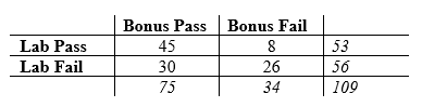
The example for this test comes from a previous semester’s STAT 217 grades. In the semester in question, the professor offered the students a “bonus test” after their midterms. This was done by allowing the students to essentially re-take the midterm given in class, but doing so on their own time and using all the resources they wanted to. A (small) fraction of the points they would earn on this bonus test would be added to their actual in-class test points.
I wanted to determine if the proportion of students who passed the lab test and failed the bonus test was equal to the proportion of students who failed the lab test but passed the bonus test, using n = 109 students and α = 0.05.
H0: πpass/fail = πfail/pass
Ha: πpass/fail ≠ πfail/pass
The following table shows the breakdown for the four possible outcomes in this case.
Computations:
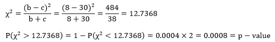
Since our p-value is smaller than our alpha-level, we reject H0 and claim that the proportions for cells b and c are significantly different.
Example in R
Since the calculations for this week’s test are quite easy, it’s probably faster to do them by hand than use R!
Week 23: The Wilcoxon Matched-Pairs Signed-Ranks Test
Yo! Today we’re going to talk about another nonparametric test: the Wilcoxon matched-pairs signed-ranks test!
When Would You Use It?
The Wilcoxon matched-pairs signed-ranks test is a nonparametric test used to determine if two dependent samples represent two different populations.
What Type of Data?
The Wilcoxon matched-pairs signed-ranks test requires ordinal data.
Test Assumptions
- The sample of subjects has been randomly selected from the population it represents.
- The original scores obtained for the subjects in the study are interval or ratio data.
- The distribution of the difference of the scores in the populations represented by the samples is symmetric about the median population difference score.
Test Process
Step 1: Formulate the null and alternative hypotheses. The null hypothesis states that in the two populations represented by the two samples, the median difference score between the two populations is zero. The alternative hypothesis claims otherwise (that the population median difference is greater than, less than, or simply not equal to zero).
Step 2: Compute the test statistic. The test statistic here is called the Wilcoxon T test statistic. Since the calculation is best demonstrated with data, please see the example shown below to see how this is done.
Step 3: Obtain the critical value. Unlike most of the tests we’ve done so far, you don’t get a precise p-value when computing the results here. Rather, you calculate your T test statistic value and then compare it to a specific value. This is done using a table (such as the one here). Find the number at the intersection of your sample size and the specified α-level. Compare this value with your T value.
Step 4: Determine the conclusion. If the calculated T value is larger than the table value, fail to reject the null hypothesis (that is, retain the claim that the samples do not represent different populations). If the calculated T value is equal to or smaller than the table value, reject the null hypothesis in favor of the alternative.
Example
The example for today’s test comes from one of the STAT 213 lab sections I taught last semester. I wanted to see if the students’ ranks in relation to their lab peers changed between midterm 1 and midterm 2. Set α = 0.05. The data is summarized in the following table, and an explanation of the columns can be found below.
H0: θD = 0
Ha: θD ≠ 0

Column 1 is the student ID.
Column 2 is the student’s ranks on midterm 1, with “1” corresponding to the student with the highest grade and “23” corresponding to the student with the lowest grade.
Column 3 is the student’s ranks on midterm 2, with “1” corresponding to the student with the highest grade and “23” corresponding to the student with the lowest grade.
Column 4 is the differences between the rank on midterm 1 and the rank on midterm 2.
Column 5 is the absolute values of Column 4.
Column 6 is the ranks of the values in Column 5. If a Column 5 value is zero, it is not ranked. If there are multiple identical values in Column 5, the average of their ranks is assigned to each of those values for Column 6.
Column 7 is the signed ranks of the values in Column 5. It is the same as Column 6, except if a value was negative in Column 4, its rank becomes negative in Column 7.
To obtain the Wilcoxon T test statistic, find the sum of the positive signed ranks and the sum of the negative signed ranks (all in Column 7). The absolute value of the smaller of these sums is the Wilcoxon T. Here,
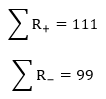
So T = 99. The table value for a two-tailed test with n = 23 and α = 0.05 is 73. Since our calculated T is larger than the critical value, we fail to reject the null hypothesis and claim that the median difference in rank in the population is not different between midterm 1 and midterm 2.
Example in R
No R example this week, as this is probably easier to do by hand.
Week 22: The t Test for Two Dependent Samples
Today we’re going to talk about our first test involving dependent samples: the t test for two dependent samples!
When Would You Use It?
The t test for two dependent samples is a parametric test used to determine if two dependent samples represent two populations with different mean values.
What Type of Data?
The t test for two dependent samples requires interval or ratio data.
Test Assumptions
- If each sample contains the same subjects (e.g., a setup that involves testing subjects at time A and then again at time B), order effects must be controlled for.
- If a matched subjects design is employed, within each pair of matched subjects, the two subjects must be randomly assigned to one of the two experimental conditions.
Test Process
Step 1: Formulate the null and alternative hypotheses. The null hypothesis claims that the two sample means are equal. The alternative hypothesis claims otherwise (one population mean is greater than the other, less than the other, or that the means are simply not equal).
Step 2: Compute the t-score. The t-score is computed as follows:

Step 3: Obtain the p-value associated with the calculated t-score. The p-value indicates the probability of a difference in the two sample means that is equal to or more extreme than the observed difference between the sample means, under the assumption that the null hypothesis is true.
Step 4: Determine the conclusion. If the p-value is larger than the prespecified α-level, fail to reject the null hypothesis (that is, retain the claim that the population means are equal). If the p-value is smaller than the prespecified α-level, reject the null hypothesis in favor of the alternative.
Example
For the data for this example, I decided to compare the age at which the internet thought I would die in 2011 to the age at which the internet thinks I would die in 2016. That is, I took 8 different online “death tests” in 2011, then re-took them this evening. The data are in the following table:

I wanted to see if there was a significant difference in the average “age of death” between 2011 and 2016, based on what information I gave these tests. Here, n = 8. Set α = 0.05.
H0: µ2011 = µ2016 (or µ2011 – µ2016 = 0)
Ha: µ2011 ≠ µ2016 (or µ2011 – µ2016 ≠ 0)
Computations:
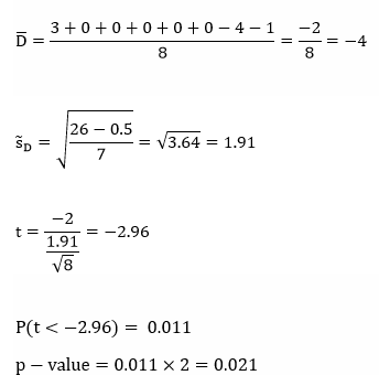
Since our p-value is smaller than our alpha-level, we reject H0 and claim that the population means are significantly different (with evidence in favor of the mean being higher in 2011).
Example in R
dat=read.table('clipboard',header=T) #"dat" is the name of the imported raw data

diffs = y2011 - y2016

n=length(diffs)

D = sum(diffs)

sdev = sd(diffs)

t = D/(sdev/sqrt(n))        #t score

pval = pt(t, n-1)*2         #p-value

                               #pt calculates the left-hand area

                               #multiply by two because it is a two-sided test
(Here’s a list of the tests, by the way.)
Week 21: The z Test for Two Independent Proportions
Hello, all! Today we’re going to talk about a two sample test involving proportions. Specifically, we’re going to talk about the z test for two independent proportions!
When Would You Use It?
The z test for two independent proportions is a nonparametric test used to determine if, in a 2 x 2 contingency table, the underlying populations represented by the samples have equal proportions of observations in one of the two categories of the dependent variable.
What Type of Data?
The z test for two independent proportions requires categorical or nominal data.
Test Assumptions
- The data represent a random sample of independent observations.
Test Process
Step 1: Formulate the null and alternative hypotheses. The data appropriate for this type of test is usually summarized in a 2 x 2 table (see the example below to get a better understanding of this). The null hypothesis claims that for the category of interest of the dependent variable, the proportion of observations from the first category of the independent variable that belong to the category of interest is equal to the proportion of observations from the second category of the independent variable that belong to the category of interest.
Step 2: Compute the test statistic. The test statistic here is a z-score and is computed as follows:

Step 3: Obtain the p-value associated with the calculated z-score. The p-value indicates the probability of observing a difference in proportions as extreme or more extreme than the observed sample difference, under the assumption that the null hypothesis is true.
Step 4: Determine the conclusion. If the p-value is larger than the prespecified α-level, fail to reject the null hypothesis (that is, retain the claim that the proportions are equal in both groups of the independent variable). If the p-value is smaller than the prespecified α-level, reject the null hypothesis in favor of the alternative.
Example
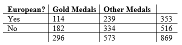
For today’s example, I wanted to see if there was a significant difference in the proportion of gold medals for European countries versus the rest of the world in the 2012 London Summer Olympics. I sampled a total of 55 countries (all countries that won at least one gold medal), then tallied the number of gold medals, the number of non-gold medals, and whether or not the country was in Europe. This data is summarized in the following table:
Let’s test the claim that the proportion of gold medals for European and non-European countries is different. Set α = 0.05.
H0: π1 = π2
Ha: π1 ≠ π2
Here, n1 = 353, n2 = 516, p1 = 0.323, and p2 = 0.353. The values of p and z and the resulting p-value are calculated as:
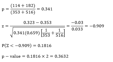
Since our p-value is larger than our alpha-level (0.3632 > 0.05), we fail to reject H0 and claim that the proportions are equal in the population.
Example in R
This example assumes that your data are in columns, with one column containing the number of gold medals per country, one column containing the number of total medals per country, and one coded column telling you whether a country belongs to Europe or not.
dat=read.table('clipboard', header=T) #'dat' is the name of the imported raw data
euro = subset(dat,europe == "y")
non = subset(dat,europe == "n")
a = sum(euro$gold)
b = sum(euro$total) - a
c = sum(non$gold)
d = sum(non$total) - c
n1 = sum(a + b)
n2 = sum(c + d)
goldsum = sum(dat$gold)
othersum = sum(total)
p1= a/n1
p2 = c/n2
p = (a + c)/(n1 + n2)
z = (p1 - p2)/(sqrt((p*(1-p))*((1/n1)+(1/n2))))
pval = (pnorm(z))*2          #p-value
                               #pnorm calculates the left-hand area
                               #multiply by two because it is a two-sided test
Week 20: The Chi-Square Test of Independence
Hello, people! Today we’re going to talk about another chi-square test: the chi-square test of independence!
When Would You Use It?
The chi-square test of independence is a nonparametric test used to determine if the two variables represented in a contingency table are independent of one another.
What Type of Data?
The chi-square test of independence requires categorical or nominal data.
Test Assumptions
- The data represent a random sample of independent observations.
- The expected frequency of each cell in the contingency table is at least 5.
Test Process
Step 1: Formulate the null and alternative hypotheses. The data appropriate for this type of test is usually summarized in an r x c table, where r is the number of rows of the table and c is the number of columns of the table (see the example below to get a better understanding of this). The null hypothesis claims that the in the population from which the sample was drawn, the observed frequency of each cell in the table is equal to the respective expected frequencies of each cell in the table. The alternative hypothesis claims that for at least one cell, the observed and expected frequencies are different.
Step 2: Compute the test statistic. The test statistic here, unsurprisingly, a chi-square value. To compute this value, use the following equation:

Eij, the expected cell count for the ijth cell, is calculated as follows:
Step 3: Obtain the critical value. The critical value can be obtained using a chi-square table (such as this one here). Find the column corresponding to your specified alpha-level, then find the row corresponding to your degrees of freedom. The degrees of freedom is calculated as df = (r – 1)(c – 1), where r is the number of rows in the table and c is the number of columns in the table. Compare your obtained chi-square value to the value at the intersection of your selected alpha-level and degrees of freedom.
Step 4: Determine the conclusion. If your test statistic is equal to or greater than the table value, reject the null hypothesis. If your test statistic is smaller than the table value, fail to reject the null (that is, claim that the observed cell frequencies match those of the expected cell frequencies).
Example
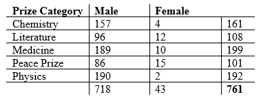
The example I’ll use today involves looking at some Nobel Prize data. Specifically, I want to see if the category of Nobel Prize (chemistry, physics, etc.) is independent of gender. The data come from here. The sample size I used was n = 761; I omitted organizations who had won the award and just looked at individuals. I also chose to omit the “Economics” category, as that had been the most recently added and did not have a lot of observations for either gender yet. Set α = 0.05.
H0: Nobel Prize category is independent of gender
Ha: Nobel Prize category is not independent of gender
Observed counts are in the following table:
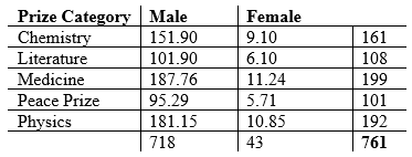
The expected cell counts, as calculated by the Eij formula above, are displayed in the following table:
Calculating the chi-square value gives us:

The degrees of freedom for this test is df = (5 – 1)(2 – 1) = 4, which gives us a critical chi-square value of 9.488 by the table. Since our calculated chi-square value, 32.894, is larger than the table value, this suggests that we reject the null and claim that prize category and gender are not independent.
Week 19: The Chi-Square Test for Homogeneity
What’s up, y’all? Today we’re going to talk about the chi-square test for homogeneity!
When Would You Use It?
The chi-square test for homogeneity is a nonparametric test used to determine whether or not r independent samples, categorized on a single dimension, are homogeneous with respect to the proportion of observations in each of the c categories.
What Type of Data?
The chi-square test for homogeneity requires categorical or nominal data.
Test Assumptions
- The data represent a random sample of independent observations.
- The expected frequency of each cell in the contingency table is at least 5.
Test Process
Step 1: Formulate the null and alternative hypotheses. The data appropriate for this type of test is usually summarized in an r x c table, where r is the number of rows of the table and c is the number of columns of the table (see the example below to get a better understanding of this). The null hypothesis claims that the in the population from which the sample was drawn, the observed frequency of each cell in the table is equal to the respective expected frequencies of each cell in the table. The alternative hypothesis claims that for at least one cell, the observed and expected frequencies are different.
Step 2: Compute the test statistic. The test statistic here, unsurprisingly, a chi-square value. To compute this value, use the following equation:
Eij, the expected cell count for the ijth cell, is calculated as follows:
Step 3: Obtain the critical value. The critical value can be obtained using a chi-square table (such as this one here). Find the column corresponding to your specified alpha-level, then find the row corresponding to your degrees of freedom. The degrees of freedom is calculated as df = (r – 1)(c – 1), where r is the number of rows in the table and c is the number of columns in the table. Compare your obtained chi-square value to the value at the intersection of your selected alpha-level and degrees of freedom.
Step 4: Determine the conclusion. If your test statistic is equal to or greater than the table value, reject the null hypothesis. If your test statistic is smaller than the table value, fail to reject the null (that is, claim that the observed cell frequencies match those of the expected cell frequencies).
Example
The example for this test comes from Amazon. Specifically, I want to see if the number of 4+ star ratings was homogeneous across the six different price ranges for laptop computers. I chose a random sample of n = 15 from each of the six price ranges and determined how many of the 15 laptops selected had four or more stars for their average review. The observed counts are in the following table:
Set α = 0.05.
H0: The proportion of 4+ star ratings is homogeneous across all price ranges
Ha: The proportion of 4+ star ratings is not homogeneous across all price ranges
The expected cell counts, as calculated by the Eij formula above, are displayed in the following table:
Calculating the chi-square value gives us:
The degrees of freedom for this test is df = (6 – 1)(2 – 1) = 5, which gives us a critical chi-square value of 11.070 by the table. Since our calculated chi-square value, 3.54, is smaller than the table value, this suggests that we fail to reject the null and claim that the proportion of 4+ star ratings is the same for each price category.
Week 18: The Siegel-Tukey Test for Equal Variability
Today we’re going to talk about another nonparametric test: the Siegel-Tukey test for equal variability!
When Would You Use It?
The Siegel-Tukey test for equal variability is a nonparametric test used to determine if two independent samples represent two populations with different variances.
What Type of Data?
The Siegel-Tukey test for equal variability requires ordinal data.
Test Assumptions
- Each sample is a simple random sample from the population it represents.
- The two samples are independent.
- The underlying distributions of the samples have equal medians.
Test Process
Step 1: Formulate the null and alternative hypotheses. The null hypothesis claims that the two population variances are equal. The alternative hypothesis claims otherwise (one variance is greater than the other, or that they are simply not equal).
[Note that from here on out, the calculations are exactly the same as for the Mann-Whitney U test. The only thing that differs is how the data are ranked.]
Step 2: Compute the test statistics: U1 and U2. Since this is best done with data, please see the example shown below to see how this is done.
Step 3: Obtain the critical value. Unlike most of the tests we’ve done so far, you don’t get a precise p-value when computing the results here. Rather, you calculate your U values and then compare them to a specific value. This is done using a table (such as the one here). Find the number at the intersection of your sample sizes for both samples at the specified alpha-level. Compare this value with the smaller of your U1 and U2 values.
Step 4: Determine the conclusion. If your test statistic is equal to or less than the table value, reject the null hypothesis. If your test statistic is greater than the table value, fail to reject the null (that is, claim that the variances are equal in the population).
Example
Today’s data come from my 2012 music selection. I wanted to see if the median play counts for two genres—pop and electronic—were the same. I chose these two because I think most of my favorite songs are of one of the two genres. To keep things relatively simple for the example, I sampled n = 8 electronic songs and n = 8 pop songs. Set α = 0.05.
H0: σ2pop = σ2electronic
Ha: σ2pop ≠ σ2electronic
The following table shows several different columns of information. I will explain the columns below.
Column 1 is the genre of each song.
Column 2 is the play count for each song, ranked from least to greatest
Column 3 is the rank of each play count. In order to obtain the ranks for this test, start by giving a rank of “1” to the lowest play count value. Then a rank of “2” to the highest play count value, a rank of “3” to the second highest play count value, a rank of “4” to the second lowest play count value, etc. (that is, assign ranks by alternating from one extreme to the other).
To compute U1 and U2, use the following equations:

So here,

The test statistic itself is the smaller of the above values; in this case, they’re both the same, so we get U = 32. In the table, the critical value for n1 = 8 and n2 = 8 and α = 0.05 for a two-tailed test is 13. Since U > 13, we fail to reject the null and retain the claim that the population variances are equal.
Example in R
No R example this week; most of this is easy enough to do by hand for a small-ish sample.
Week 17: The Moses Test for Equal Variability
Today we’re going to talk about another nonparametric test: the Moses Test for equal variability!
When Would You Use It?
The Moses Test for equal variability is a nonparametric test used to determine if two independent samples represent two populations with different variances.
What Type of Data?
The Moses Test for equal variability requires ordinal data.
Test Assumptions
- Each sample is a simple random sample from the population it represents.
- The two samples are independent.
Test Process
Step 1: Formulate the null and alternative hypotheses. The null hypothesis claims that the two population variances are equal. The alternative hypothesis claims otherwise (one variance is greater than the other, or that they are simply not equal).
Step 2: Compute the test statistics: U1 and U2. Since this is best done with data, please see the example shown below to see how this is done. [Note that the test statistic calculations are exactly the same as for the Mann-Whitney U test. The only thing that differs is the ranking procedure.]
Step 3: Obtain the critical value. Unlike most of the tests we’ve done so far, you don’t get a precise p-value when computing the results here. Rather, you calculate your U values and then compare them to a specific value. This is done using a table (such as the one here). Find the number at the intersection of your sample sizes for both samples at the specified alpha-level. Compare this value with the smaller of your U1 and U2 values.
Step 4: Determine the conclusion. If your test statistic is equal to or less than the table value, reject the null hypothesis. If your test statistic is greater than the table value, fail to reject the null (that is, claim that the variances are equal in the population).
Example
Today’s data come from my 2012 music selection (I’ll use this data next week, too!). I wanted to see if the median play counts for two genres—pop and electronic—were the same. I chose these two because I think most of my favorite songs are of one of the two genres. To keep things relatively simple for the example, I sampled n = 8 electronic songs and n = 8 pop songs. Set α = 0.05.
H0: σ2pop = σ2electronic
Ha: σ2pop ≠ σ2electronic
Here are the raw data:

The following tables show several different columns of information. I will explain the columns below.

The “Subsample” column: to obtain the rankings for this test, first divide the n1 scores in sample 1 into m1 subsamples (m1 > 1), with each subsample comprised of k scores. Then divide the n2 scores of sample 2 into m2 subsamples (m2 >2), with each subsample comprised of k scores. To form the subsamples, employ sampling without replacement within each of the samples. Ideally, m1, m2, and k should be chosen such that (m1)(k) = n1 and (m2)(k) = n2 if at all possible. Here, m1 = m2 = 4, and k = 2. The “subsample” columns list the four subsamples of play counts for each genre.
The second column contains the average of the k values for a given subset. It’s just the average of the values in the “subsample” column.
The third column contains the differences between each subsample value (X) and the subsample’s mean.
The fourth column is just the third column’s values squared.
The fifth column contains the sum of the values in the fourth column.
The sixth column contains the rank of the value in the fifth column over both genres. The smallest values is ranked as 1 and the largest is ranked as 8 (in this case).
To compute U1 and U2, use the following equations:

So here,
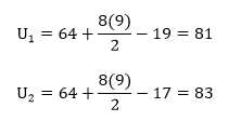
The test statistic itself is the smaller of the above values, so we get U = 81. In the table, the critical value for n1 = 8 and n2 = 8 and α = 0.05 for a two-tailed test is 13. Since U > 13, we fail to reject the null and retain the claim that the population variances are equal.
Example in R
x=read.table('clipboard', header=T)              #data
attach(x)
elects=subset(x,genre=="Electronic")
pops=subset(x,genre=="Pop")
group1=matrix(rep(NaN,8),nrow=4)
group2=matrix(rep(NaN,8),nrow=4)


group1=as.matrix(sample(elects[,2],8,replace=F)) #subgroups for sample 1
sub1.1=group1[1:2,]
sub1.2=group1[3:4,]
sub1.3=group1[5:6,]
sub1.4=group1[7:8,]


group2=as.matrix(sample(pops[,2],8,replace=F))   #subgroups for sample 1
sub2.1=group2[1:2,]
sub2.2=group2[3:4,]
sub2.3=group2[5:6,]
sub2.4=group2[7:8,]
samps=rbind(sub1.1,sub1.2,sub1.3,sub1.4,sub2.1,sub2.2,sub2.3,sub2.4)


xbars=rep(NaN,8)                                 #column 2
for(i in 1:8){
xbars[i]=mean(samps[i,])}
xbars=as.matrix(xbars)


diffs1=rep(NaN,8)                                #column 3
for(i in 1:8){
diffs1[i]=(samps[i,1]-xbars[i])}
diffs2=rep(NaN,8)
for(i in 1:8){
diffs2[i]=(samps[i,2]-xbars[i])}


diffs=cbind(diffs1,diffs2)                       #column 4


diffs2=diffs^2                                   #column 5


sumdif=rep(NaN,8)
for(i in 1:8){
sumdif[i]=diffs2[i,1]+diffs2[i,2]}               #column 6
Week 16: The Kolmogorov-Smirnov Test for Two Independent Samples
[This is coming out on a Monday ’cause I was super busy yesterday and had no time to make this/post it.]
Today’s test is a non-parametric test for two samples: the Kolmogorov-Smirnov test for two independent samples!
When Would You Use It?
The Kolmogorov-Smirnov test for two independent samples is a nonparametric test used to determine if two independent samples represent two different populations.
What Type of Data?
The Kolmogorov-Smirnov test for two independent samples requires ordinal data.
Test Assumptions
- All of the observations in the samples are randomly selected and independent of one another.
- The scale of the measurement is ordinal.
Test Process
Step 1: Formulate the null and alternative hypotheses. The null hypothesis claims that the the distribution underlying the population for one sample is the same as the distribution underlying the population for the other sample. The alternative claims that the distributions are not the same.
Step 2: Compute the test statistic. The test statistic, in the case of this test, is defined by the point that represents the greatest vertical distance at any point between the cumulative probability distribution constructed from the first sample and the cumulative probability distribution constructed from the second sample. I will refer you to the example shown below to show how these calculations are done in a specific testing situation.
Step 3: Obtain the critical value. Unlike most of the tests we’ve done so far, you don’t get a precise p-value when computing the results here. Rather, you calculate your test statistic and then compare it to a specific value. This is done using a table. Find the number at the intersection of your sample sizes for your specified alpha-level. Compare this value with your test statistic.
Step 4: Determine the conclusion. If your test statistic is equal to or larger than the table value, reject the null hypothesis (that is, claim that the distribution of the data is inconsistent with the hypothesized population distribution). If your test statistic is less than the table value, fail to reject the null.
Example
For this test’s example, I want to use some of my music data from 2012. I know that I tend to listen to music from the “electronic” genre and from the “dance” genre fairly equally, so I want to determine, based on play count, if I can say that the population distributions for these genres are similar. To keep things simple, I will use nelectronic = 6 and ndance = 6.
H0: Felectronic(X) = Fdance(X) for all values of X
Ha: Felectronic(X) ≠ Fdance(X) for at least one value of X
Computations:
For the computations section of this test, I will display a table of values for the data and describe what the values are and how the test statistic is obtained.

Column A and Column C, together, show the ranked values of the play counts for electronic (Column A) and dance (Column C).
Column B represents the cumulative proportion in the sample for each play count in Column A. For example, for the play count = 7, the cumulative proportion of that value is just 1/6, since there is no smaller value in Column A.
Column D represents the same thing as column B, except for Column C.
Column E is Column B – Column D.
The test statistic is obtained by determining the largest value from Column E. Here, the test statistic is .5. This value is compared to the critical value at α = 0.05, n1 = 6, n2 = 6, which is .667. Since our test statistic is not larger than our critical value, we fail to reject the null and claim that the distributions of play counts for electronic and dance are similar.
Example in R
No R example this week, as this is pretty easy to do by hand, especially with having to rank things.
Week 15: The Mann-Whitney U Test
Today we’re going to talk about another nonparametric test: the Mann-Whitney U test!
When Would You Use It?
The Mann-Whitney U test is a nonparametric test used to determine if two independent samples represent two populations with different medians.
What Type of Data?
The Mann-Whitney U test requires ordinal data.
Test Assumptions
- Each sample is a simple random sample from the population it represents.
- The two samples are independent.
- The original scores obtained are continuous random variables (which are later ranked).
- The underlying distributions of the samples are identical in shape (but do not necessarily have to be normal).
Test Process
Step 1: Formulate the null and alternative hypotheses. The null hypothesis claims that the two population medians are equal. The alternative hypothesis claims otherwise (one median is greater than the other, or that they are simply not equal).
Step 2: Compute the test statistics: U1 and U2. Since this is best done with data, please see the example shown below to see how this is done.
Step 3: Obtain the critical value. Unlike most of the tests we’ve done so far, you don’t get a precise p-value when computing the results here. Rather, you calculate your U values and then compare them to a specific value. This is done using a table (such as the one here). Find the number at the intersection of your sample sizes for both samples at the specified alpha-level. Compare this value with the smaller of your U1 and U2 values.
Step 4: Determine the conclusion. If your test statistic is equal to or less than the table value, reject the null hypothesis. If your test statistic is greater than the table value, fail to reject the null (that is, claim that the medians are equal in the population).
Example
Today’s data come from my 2012 music selection. I wanted to see if the median play counts for two genres—pop and electronic—were the same. I chose these two because I think most of my favorite songs are of one of the two genres. To keep things relatively simple for the example, I sampled n = 8 electronic songs and n = 8 pop songs. Set α = 0.05.
H0: θpop = θelectronic
Ha: θpop ≠ θelectronic
The following table shows several different columns of information. I will explain the columns below.

Column 1 is the genre of each song.
Column 2 is the play count for each song.
Column 3 is the overall rank of the play count, regardless of which genre it came from.
If there had been ties, I would have summed the number of ranks that were taken by the ties, and then divide that value by the number of ties.
To compute U1 and U2, use the following equations:
So here,

The test statistic itself is the smaller of the above values; in this case, we get U = 28. In the table, the critical value for n1 = 8 and n2 = 8 and α = 0.05 for a two-tailed test is 13. Since U > 13, we fail to reject the null and retain the claim that the population medians are equal.
Example in R
No R example this week; most of this is easy enough to do by hand for a small-ish sample.

