TWSB: Hear Me Out
DID YOU KNOW: the loudest a sound can be (on earth) is 194 decibels?
By definition, something that is 0 dB is giving off a sound that is just detectable to the human ear. Softer sounds get negative dBs, louder sounds get positive dBs. A 10 dB increase corresponds to a doubling in loudness, meaning that, for example, something that is 30 dB is twice as loud as 20 dB and three times as loud as 10 dB.
So why is the upper limit the very specific loudness of 194 dB? Because sound is vibration. More specifically, it’s longitudinal waves. It’s like if you took a slightly stretched slinky, laid it out straight, and then rapidly pushed in and pulled back on one end of the slinky. The compressed metal spirals would move along the slinky’s body. That’s a longitudinal wave form.
For sound, this “compressed slinky” is compressed air (or whatever medium we’re in) and the compressed parts are parts of higher pressure (the expanded parts are parts of lower pressure).
Once we’re to the point that we’re hitting 194 dB, we’re at the threshold where this pressure wave switches to a shock wave. The energy is no longer moving through the air but is instead pushing the air outward. The “wave” becomes so extreme that the low pressure regions no longer have any molecules of air left in them to continue the push of the wave. All the molecules just move outward at once. It’s no longer technically sound as we define it in wave form. For example, the atomic bombs dropped on Hiroshima and Nagasaki were likely well over 200 dB and thus created shockwaves.
Also, if a shockwave is strong enough, it can freaking liquify you.
Isn’t that fascinating?
One of my old NaNoWriMo projects was about some guys trying to engineer the perfect sound that would resonate with the human body, but they get hooked on the euphoria they experience by this sound and continue to increase its intensity and volume and eventually kill themselves with it.
Y’know, just another one of my cheerful NaNo topics.
Anyway. Super cool, huh?
TWSB: More on the Kilogram
So I have no idea how I’ve never found this podcast before since it’s about the kilogram, but I haven’t.
But now I have.
Enjoy.
(Hot damn, I love the kilogram.)
This Week’s (Month’s?) Science Blog: Sun Block
Yo.
So as you all know, I find the sun to be very awesome. Here’s a video of a guy demonstrating that despite the fact that the sun seems so huge in our sky a lot of the time, that hugeness is an illusion! The sun is, in fact, only about half a degree in size in our sky.
Supah cool.
TWSB: Hey, A Science Blog!
Hey you butt parties, check this out: a study published in the journal Chemical Senses suggests that there may be a sixth taste in addition to the five basic ones we all know (sweet, sour, salty, bitter, umami). What taste is it? Starch.
The study, run by Dr. Juyun Lim from OSU, involved approximately 100 participants across five different studies. The participants were asked to taste liquid solutions of carbohydrates—some simple (like sugar) and some complex—both under normal conditions and when the sweet receptors in their mouths were blocked. Even with the receptors blocked, the participants stated that they could still detect a starchy taste, which goes against previous assumptions that starch was tasteless.
Dr. Lim says that the result is not necessarily surprising; since humans use starch as a major source of energy, it makes sense that humans could be able to detect its presence by taste. If nothing else, the findings demonstrate that the way humans taste is actually more complex than previously thought. The way the participants tasted the starch, says Dr. Lim, was by tasting the saliva-destroyed version of the starch: glucose oligomers. While it was previously suggested that humans could only taste the simple sugars class of carbohydrates, the fact that participants could actually describe the taste of the glucose oligomers suggests that our tasting of carbs is more complicated than we think.
Others are a bit wary of classifying this as a new separate taste, suggesting that it might just be another “version” of the sweet taste. More research will be done on determining the exact mechanism of how the glucose oligomers are actually tasted.
TWSB: Blacker than the Blackest Black Times Infinity (Part II)
I did a post quite a while ago on super black material, but it looks like they’ve recently come up with something that’s even blacker.
Surrey NanoSystems, a British company, have improved their Vantablack material so that it absorbs more than 99.96% of the light that hit it—more than their original Vantablack, which had first been created in 2014. In fact, the new material absorbs so much light that scientists are unable to measure exactly how black the material is. You can shine a laser pointer onto it and the laser seems to disappear.
Vantablack is made by packing carbon nanotubes so tightly together that light can get in but can’t escape. Here’s a crumpled up piece of aluminum foil painted with Vantablack.
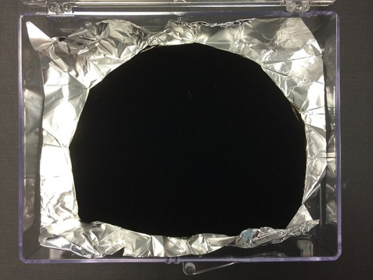
Freaky, huh?
This Week’s Science Blog: Remember When I Used to do a Weekly Science Blog?
SUN NEWS!
According to research at the University of Warwick, the sun may have the potential to superflare. What’s a superflare? It’s supercool. Superflares are like solar flares, only thousands of times more powerful. According to the lead researcher at Warwick, Chloe Pugh, if the sun were to superflare, pretty much all of earth’s communications and energy systems could fail. Radio signals disabled, huge blackouts, all that fun stuff. But according to Pugh, the conditions needed for a superflare are extremely unlikely to occur on the sun.
But how did they actually figure out that it is possible for the sun to superflare? Using NASA’s Kepler space telescope, the researchers found a binary star, KIC9655129, which has been shown to superflare. The researchers suggest that due to the similarities between the sun’s solar flares and the superflares of KIC9655129, the underlying physics of both phenomena may be the same.
Cool!
TWSB: The Problem with Pentagons
Well this is cool. Apparently, a group of mathematicians have recently found a new type of pentagon that can tile the plane—meaning that it can cover the plane leaving no gaps and having no overlaps. It is the 15th type of pentagon known to be able to tile the plane and the first discovered in 30 years.
Apparently searching for tiling pentagons has been a thing for about a century now. Karl Reinhardt, back in 1918, discovered five classes of pentagons that tile the plane. These five were considered all the possible tiling pentagons until 1968, when three more were found. The list continued to grow until about 30 years ago, when it stalled at 14 types of pentagons. Until now!
The discovery was made by Casey Mann, Jennifer McLoud, and David Von Derau. The three, working at the University of Washington Bothell, used a computer to search through a finite set of possibilities.
Why so much interest in tiling pentagons? Well, it turns out that pentagons are the only one of the “-gons” that isn’t completely understood. For example, all triangles and quadrilaterals have been classified as being able to tile the plane, exactly three types of (convex) hexagons tile the plane, and no other –gon is able to tile the plane. But pentagons haven’t been fully classified yet.
So the research must press on! There may end up being more tilings that are discovered, but for now, have a picture of the 15 pentagon shapes known to tile the plane (with the most recent one in the bottom right corner) (picture from article linked above):

This Week’s Science Blog is Cheesy
Always a good topic, huh?
In the Scientific American article linked above, author Steve Mirsky talks about how a decades-old Swiss genetic experiment on flies is related to a more current set of experiments regarding what causes the formation and development of the eyes (or holes) in Emmental (or Swiss) cheese.
In the fly experiment, geneticists managed to get a fly to grow a ton of eyes all over its body by isolating and manipulating a few of the fly’s genes. More recently, 13 researchers at three different Swiss research facilities have figured out the link between the genetic fiddling needed to create the extra fly eyes and the genetic fiddling needed to regulate the size and quantity of holes in Swiss cheese.
The study, published as “Mechanism and Control of the Eye Formation in Cheese,” was published in the International Dairy Journal and contains a discussion on why eye/hole regulation is important.
“The size of the eyes of first-quality cheese should be between the size of a cherry … and a walnut,” says the journal article. However, different cheese-lovers prefer different sizes (and quantities) of eyes. “Italian consumers prefer Emmental cheese with walnut-sized eyes, whereas commercial manufacturers of sliced cheeses ask for cheese with smaller eyes and higher eye numbers.”
In making cheese, bacteria is key. A product of the bacteria is carbon dioxide, which forces the holes to expand to any given size, but until this study, it was unknown what made the holes themselves begin to form in the first place. Turns out, the process is analogous to the process of how a raindrop forms around a particle (a “cloud condensation nuclei”) in the vapor-saturated air. For the cheese, a little particle can act as an eye nucleus, around which the round hole begins to form.
In the study, the researchers chose hay dust as their particles of choice and found, through varying the amount of dust the young Swiss cheese was exposed to, that they could actually control the number and size of the eyes.
So they can basically do cloud seeding, but with cheese. Cheese seeding? Cheeding?
Anyway. Pretty cool!
TWSB: Analyzing Old Faithful with Faithful Old Regression
Alright y’all, sit your butts down…it’s time for some REGRESSION!
If you’ve ever gone to Yellowstone National Park, you likely stopped to watch Old Faithful shoot off its rather regular jet of water. In case you’ve never seen this display, have a video taken of an eruption in 2007:
(Side note: you can hear people frantically winding their disposable cameras throughout the video. Retro.)
What does Old Faithful have to do with regression, you ask?
Well, while the geyser is neither the largest nor the most regular in Yellowstone, it’s the biggest regular geyser. Its size, combined with the relative predictability of its eruptions, makes it a good geyser for tourists to check out, as park rangers are able to estimate when the eruptions might occur and thus inform people about them. And that’s where regression comes into play: by analyzing the relationship between the length of an Old Faithful eruption and the waiting time between eruptions, a regression equation can be created that can allow for someone armed with the length of the last eruption to predict the amount of waiting time until the next one. Let’s see how it’s done!*
Part 1: What is Regression?
(This is TOTALLY not comprehensive; it’s just a very brief description of what regression is. There are a lot of assumptions that must be met and a lot of little details that I left out, but I just wanted to give a short overview for anyone who’s like, “I know a little bit about what regression is, but I need a bit of a refresher.”)
Regression is a statistical technique used to describe the relationship between two variables that are thought to be linearly related. It’s a little like correlation in the sense that it can be used to determine the strength of the linear relationship between the variables (think of the relationship between height and weight; in general, the taller someone is, the more they’re likely to weigh, and this relationship is pretty linear). However, unlike correlation, regression requires that the person interested in the data designate one variable as the independent variable and one as the dependent variable. That is, one variable (the independent variable) causes change in the other variable (the dependent variable, “dependent” because its value is at least in part dependent on the changes of the independent variable). In the height/weight example, we can say that height is the independent variable and weight the dependent variable, as it makes intuitive sense to say that height affects weight (and it doesn’t really make sense to say that weight affects height).
What regression then allows us to do with these two variables is this: say we have 30 people for which we’ve measured both their heights and weights. We can use this information to construct an equation of a line—the regression line—that best describes the linear relationship between height and weight for these 30 people. We can then use this equation for inference. For example, say you wanted to estimate the weight for a person who was 6 feet tall. By plugging in the value of six feet into your regression equation, you can calculate the likely associated weight estimate.
In short, regression lets us do this: if we have two variables that we suspect have a linear relationship and we have some data available for those two variables, we can use the data to construct the equation of a line that best describes the linear relationship between the variables. We can then use the line to infer or estimate the value of the dependent variable based on any given value of the independent variable.
Part 2: Regression and Old Faithful
We can apply regression to Old Faithful in a useful way. Say you’re a park ranger at Yellowstone and you want to be able to tell tourists when they should start gathering around Old Faithful to watch it spout its water. You know that there’s a relationship between how long each eruption is and the subsequent waiting time until the next eruption. (For the sake of this example, let’s say you also know that this relationship is linear…which it is in real life.) So you want to create a regression equation that will let you predict waiting time from eruption time.
You get your hands on some data**—recorded eruption lengths (to the nearest .1 minute) and the subsequent waiting time (to the nearest minute) and you use this to build your regression equation! Let’s pretend you know how to do this in Excel or SPSS or R or something like that. The regression equation you get is as follows:
WaitingTime = 33.97 + 10.36*EruptionTime
What does this regression equation tell us? The main thing it tells us is that based on this data set, for every minute increase in the length of the eruption (EruptionTime), the waiting time (WaitingTime) until the next eruption increases by 10.36 minutes.
It also, of course, gives us a tool for predicting the waiting time for the next eruption following an eruption of any given length. For example, say the first eruption you observe on a Wednesday morning lasts for 2.9 minutes. Now that you’ve got your regression equation, you can set EruptionTime = 2.9 and solve the equation for the WaitingTime. In this case,
WaitingTime = 33.97 + 10.36*2.9 = 33.97 + 30.04 = 64.01
That means that you estimate the waiting time until the next eruption to be a little bit more than an hour. This is information you can use to help you do your job—telling tourists when the next eruption is likely.
Of course, no regression equation (and thus no prediction based off a regression equation) is perfect—I’ve read that people who try to predict eruptions based on regression equations are usually within a 10-minute margin, plus or minus—but it’s definitely a useful tool in my opinion. Plus it’s stats, so y’know…it’s cool automatically.
END!
*I actually have no idea if Yellowstone officials actually have used regression to determine when to tell crowds to gather at the geyser; I can’t remember how it’s all even set up at the Old Faithful location, seeing as how I was like six years old when I saw it and Nate and I were thwarted in our efforts to see it a few weeks ago. But hey, any excuse to talk about stats, right?
**There are a decent number of Old Faithful datasets out there; I chose this one because it was easy to find and decently precise with regards to recording the durations.
This Week’s Science Blog: Look Up
(Hey look, it’s one of them TWSB posts! It’s been awhile, huh?)
So anybody who knows me knows I like clouds and cloud classifications, right? Well, so does (as expected) the World Meteorological Association (WMO). In fact, they published the first edition of the International Cloud Atlas in 1896 and have been updating it ever since.
Well, actually, the last update—meaning the last new cloud type added—was way back in 1951 (it was the cirrus intortus, meaning “an entangled lock of hair”).
However, thanks to people who really like to look up at the sky and try to classify all the clouds in it, there might be a new addition in the 2015 edition of the Atlas. The call for the possible new cloud type, the undulatus asperatus (“turbulent undulation”), arose in 2009 from Gavin Pretor-Pinney, a cloud enthusiast and founder of the Cloud Appreciation Society (I HAVE HIS CLOUD BOOK). He was editing selections of cloud photos for the Society’s gallery when he saw several of this new type of cloud which he believed did not fit into any other variety.
To gain further support for the new cloud type, Pretor-Penney worked with Graeme Anderson, a graduate student at the University of Reading, who wrote his dissertation on the undulates asperatus. In addition, many other cloud enthusiasts have continued to document cases of this type of cloud around the world with hopes that the WMO will officially add it in 2015.
Clouds, man.
TWSB: You Missed a (Big) Spot
Jupiter news!
So we all know the giant red spot on the giant, fast-rotating planet, right?
Of course we do! But do we know why it’s red?
For a long time, the main theory has been that the spot is red because the giant storm creating it is churning up reddish chemicals from beneath Jupiter’s clouds and bringing them to the surface for us to see.
But a new theory states that the redness of the massive swirling isn’t due to chemicals from beneath the clouds but rather due to chemical reactions with sunlight. Work by Kevin Bains, Bob Carlson, and Tom Momary, scientists based at NASA’s Jet Propulsion Laboratory, state that based on data collected from both laboratory experiments and Cassini’s flyby of the planet in 2000, they suspect that the red tint is due to the effects of ultraviolet light on ammonia and acetylene, the gases in the uppermost portion of the storm.
Baines states that if this is the case, then the spot is probably pretty dull in color beneath its uppermost clouds. According to the older theory, if the reddish chemicals are indeed coming from beneath the clouds, then the spot would be red all the way through. Baines and the others are currently doing more testing/simulations to try to gain evidence about what color lies beneath the red.
As for why the great red spot is, well, the only great red spot on the planet, Baines suggests it’s because it’s a very tall storm—much taller than any other—and thus is more likely to get “sunburnt.”
TWSB: Take Me Down Like I’m a Domino
More like TYSB (This Year’s Science Blog) since I haven’t posted one of these in forever.
Sorry. I’m a bad person.
Anyway, check out this vid:
In case you’re not the type to read the description below the video, a domino can knock over another domino that’s about 1.5 times the original domino’s size. The idea to try this came originally from scientist Lorne Whitehead in 1983.
In the video, they only use 13 dominoes. However, if they had kept making larger and larger ones, the 29th one in the tumble would have been about the size of the Empire State Building, the 62nd would be large enough to almost hit the moon (assuming, of course, that we could keep the earth’s gravity constant over all of these mega dominoes), and the 133rd would have the same length as the diameter of the Milky Way.
Reddit user Variance_on_Reddit (along with other nerdy Redditors) calculated that the time it would take these 133 dominoes to actually fall would be 11.67 quadrillion years due to friction (again, keeping “earth” conditions constant across all dominoes).
Pretty snazzy.
Reddit link (warning: Reddit)
TWSB: Twist n’…uh…Twist Again, I Guess
Meet the hemihelix!
Observed by a group of researchers at Harvard, a hemihelix occurs when a corkscrewing shape changes the direction of its spiraling. These locations are called perversions (giggity) and look like the part of the spiral being pointed at by the arrow:

(Piccy from link above)
The Harvard team observed the hemihelices when they were taking two strips of rubber of different length and stretching the shorter one to match the length of the longer one before binding them together. Unexpectedly, the hemihelix shape appeared when the tension on the joined rubber strips was released.
Understanding how and why such shapes are formed might help researchers mimic the shapes of molecules that could be used in nanotechnology. Says Dr. Katia Bertoldi, associate professor of applied math at Harvard, “Once you are able to fabricate these complex shapes and control them, the next step will be to see if they have unusual properties; for example, to look at their effect on the propagation of light.”
Cool, huh?
TWSB: C is for Complex Number, That’s Good Enough for Me
Well this is one of the coolest things I’ve ever learned about.
So I’m in Complex Variables this semester, right? Today we talked about how to take limits of complex numbers as well as the closely related topic of infinity.
I’m assuming most people who read this regularly (or just happen to stumble upon it) know at least a little about infinity in the context of real numbers. Mainly, if we represent the reals on a number line, we have a direction that goes off towards negative infinity and a direction that goes off to positive infinity. But does this translate to complex numbers?
Well, not really. When we deal with complex numbers, we deal with the complex plane: a 2-D space with one axis representing the real part of a number and the other axis representing the imaginary part of a number. That is, one way we can think of a complex number is as a set of coordinates on the complex plane. For example, if I had the number z = 3 + i2, I could represent it with the coordinates (3,2) and plot it like this:
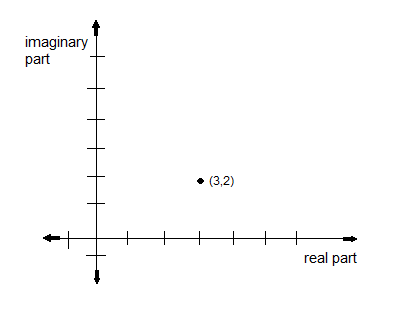
Since we’re now dealing with a plane, we actually have infinitely many directions that can be thought of as infinity—basically, any direction out from the origin.
So how do we define infinity in the complex plane to allow us to, among other things, take limits involving the point at infinity?
Answer: The Riemann sphere!
The Riemann sphere is a stereographic projection of the complex plane onto the unit sphere at the point (0,0,1). Piccy from Wiki:
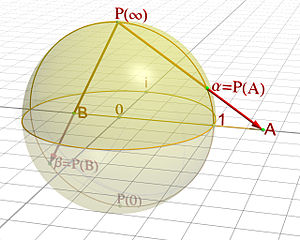
So what does this do? Well, for each point A on the complex plane, there exists a line that intersects both the point A and the north pole of the sphere. This line hits the sphere itself at α, point unique to the position of point A in the complex plane—that’s how the plane is “mapped” to the sphere and that unique mapping point is called the “projection” of point A.
The further out you go on the complex plane—that is, the further away from the sphere you go, those projection points get closer and closer to the north pole itself. However, no point is projected directly onto the north pole. So we can think of the north pole as being the image of all the points in the complex plane that are at infinity.
Isn’t that cool? It’s a way to reduce an “infinite number of infinities” to a single point.
We didn’t have time to talk about how we’re going to use it yet, but just that idea is super cool and required a blog post.
TWSB: The Sounds of Sorting
This is easily one of the coolest videos I’ve ever found on YouTube.
(note: put your speakers at a lower volume; this seemed fairly loud to me.)
A sorting algorithm is pretty much exactly what it sounds like: it’s an algorithm that puts the elements of a list in a certain order (like in the video above, where the bars represent integers and the algorithms are putting the integers in order from smallest to largest).
There are a bunch of different types, depending on what’s most important to the individual using the algorithm: ease of coding, run time, stability, etc. For example, the bubble sort (4:01 in the vid) has a fairly short code, but has a long run time compared to something like a radix sort (1:56).
At 3:11 and 3:14, you hear Pac Man!
The algorithms used in this video are, in order: selection sort, insertion sort, quick sort, merge sort, heap sort, radix sort (LSD), radix sort (MSD), std::sort (intro sort), std::stable_sort (adaptive merge sort), shell sort, bubble sort, cocktail shaker sort, gnome sort, bitonic sort and bogo sort (30 seconds of it).
How cool is this??
Here is a little code “cheat sheet” by the creator of this video, Timo Bingmann. Check out his Sound of Sorting page!
(Seriously, I’ve watched this video about 20 times already. It gives me goosebumps!)
TWSB: Swingers
Here are some pendulums:
I didn’t want the video to end!
According to the site, one complete cycle lasts 60 seconds. In that period, the longest pendulum oscillates 51 times and each successively shorter pendulum makes one additional oscillation more than the last—thus, the shortest oscillates 65 times.
I really like how when they’re all out of sync it looks like they’re slowing down and coming to a stop, but then they sync up a little again and it’s like, “BOOSH we’re still going!”
Very cool.
Somewhat unrelated, but here’s another mathy vid that I didn’t want to see the end of. Which of the three panels captured your attention the most? On the first watch it was the middle panel, on the second watch it was the far left panel for me.
TWSB: It’s Like Trying to Find a Needle in an Ionosphere
So raise your hand if you knew that in 1963, MIT launched 480,000,000 copper needles into space with the purpose of creating an artificial ionosphere.
‘Cause I sure as hell didn’t.
Wiki: “At the height of the Cold War, all international communications were either sent through undersea cables or bounced off the natural ionosphere. The United States Military was concerned that the Soviets might cut those cables, forcing the unpredictable ionosphere to be the only means of communication with overseas forces.”
And the US Military is not the US Military unless they take DRASTIC MEASURES! So up went the millions of needles. Welcome to Project West Ford.
And what makes it even better is that THEY SCREWED IT UP THE FIRST TIME SO THEY HAD TO DO IT AGAIN. “After a failed first attempt launched on October 21, 1961 (the needles failed to disperse), the project was eventually successful with the May 9, 1963 launch.”
Worldwide criticism? Yup. “British radio astronomers, together with optical astronomers and the Royal Astronomical Society, protested this action. The Soviet newspaper Pravda also joined the protests under the headline “U.S.A. Dirties Space.””
But some good did come of it: all the protesting eventually resulted in a provision about consultation in the 1967 Outer Space Treaty.
As of 2008, there were still clumps of needles out there. The needles occasionally re-enter, just as they have been since the start of the whole thing.
Just…wow.
TWSB: International Moon Station
Another demonstration of just how much “space” is in space.
Edit: Tumblr has led me to this wonderful (and slightly terrifying) video…
…as well as this info:
“What if the moon was the same distance away as the ISS? … While we think of the International Space Station as being, well, way out there in space, it’s not that far. Only around 400 km up, actually. If the Earth was a basketball, then the ISS would only be about a centimeter off its surface.
“On average, our moon resides 384,400 km away from Earth. … Even at that incredible distance, the moon can warp the liquid on the surface of Earth! Which brings me to a major problem with this video … in order to see this, we’d all be dead, and Earth would be very messed up indeed.”
TWSB: Boston Dynamics, You Scary (But Cool!)
So remember Boston Dynamics, the friendly robot constructors who brought us Little Dog, Big Dog, and Alpha Dog?
Well, now they’re switching species. Meet WildCat:
Note: it’s motoring at a max speed of 16 mph in that video.
Can you imagine being in one of those drivers on the road in the background? All you’d hear at first was something that sounded like a weed-whacker on steroids and then you’d happen to glance out the window and see this double-butted thing just booking it as it frolics in a parking lot.
Of course, if you’re driving back there, you’re probably either a Boston Dynamics employee or are at least familiar with their shenanigans, so you probably just say to yourself, “oh, there’s WildCat.”
Still, though.
TWSB: It’s That SI Unit That Won’t Conform Again
Thisiscoolthisiscoolthisiscool.
I keep coming back to the kilogram in these science blogs. One day I think I’ll do like a (somewhat) comprehensive history of the SI units, ’cause I find them fascinating.
(I also really like the word kilogram.)
TWSB: It’s Flippin’ Hot!
THIS
IS
THE
COOLEST
THING
EVER.
Are you ready to GET YO’ MIND BLOWN?
Okayokayokayokay. So you know how the earth’s magnetic field switches poles every so often? So does the sun’s!
The sun is currently at the peak of its 11 year solar cycle and is about to swap its north magnetic pole for its south and vice versa. According to Stanford University solar physicist Todd Hoeksema, the swapitself isn’t more than 3 to 4 months out. The north pole has actually already flipped; we’re just waiting on the south one to get its butt in gear and head to the opposite side.
So what does this mean for our solar system? What solar physicists focus on during this time is something called the “current sheet.” This is a surface that juts outward from the sun’s equator along which runs an electric current produced by the sun’s magnetic field. The current itself is small but the sheet is freaking huge, and it’s the thing that pretty much keeps the heliosphere (the sun’s magnetic influence) in check.
According to Phil Scherrer, another Stanford solar physicist, the sheet becomes really wavy and warped during a pole swap. So for us here on earth, as we zoom around in our orbit of the sun, we pass in and out of the sheet itself. This can cause disruptive “cosmic weather,” but the warped sheet actually offers the solar system better protection against cosmic rays.
Stanford’s Wilcox Solar Observatory has observed three such polar swaps since 1976. This will be the fourth.
HOW. COOL. IS. THAT. I freaking love the sun.
Video!
This Week’s Science Blog: DROP THE BASS! …er, Pitch.
THE PITCH DROPPED!
AND IT WAS FILMED!
WHAT THE HECK AM I YELLING ABOUT?!
In 1944, an experiment was set up that would last quite a long time. At Trinity College in Dublin, tar pitch was heated and placed into a funnel. The funnel was placed in a jar and was left alone. It’s still sitting there today. Why? Because pitch is something that, at first glance, behaves very much like a solid. It just kinda sits there and if you hit it with something hard enough, it shatters. What they wanted to show with this experiment (which is actually similar to an even longer-lived experiment done in Australia) is that, given time, pitch will exhibit liquid properties. In particular, over a (very long) stretch of time, the pitch in the funnel will succumb to gravity and drop to the bottom of the jar.
So that’s the basic idea. But the big deal in all of this is actually witnessing these drops. Averaging things out between the Australian and Dublin versions of the experiment, it takes somewhere between 7 and 13 years for the drops to happen. That’s a lot of time sitting and watching for a payoff that takes a split-second. Up until now, no one has witnessed it happening.
However, when the Dublin scientists realized last April that a drop was imminent, they did something they could finally do because of today’s technology: they set up a camera to record the pitch* when it finally fell.
And a week ago? VICTORY! On Thursday, July 11th, a pitch drop was not only witnessed, but filmed! See a gif of it here.
HOW COOL?
And we know it’ll happen again…we just need to wait.
*Actually, I think I read somewhere that they tried this in Australia in like 2000, but the camera wasn’t on when it happened. Oops.
TWSB: HIDE YO CELLPHONES, HIDE YO POWERGRIDS!
Holy solar-driven demise, Batman. Look at those enormous sunspots.
1785 and 1787—the names for these two groups of spots—are pretty much staring earth in the face right now.
Sun spots are dark areas of intense magnetic activity that, when the activity gets super-intense, spit out energy in the form of solar flares or coronal mass ejections. The flares/ejections fire out clouds of magnetic energy and solar material into space.
And what happens when these things hit earth? Normally, we end up with more extreme aurora that are able to be seen at lower latitudes. But if the storm of magnetism is really strong, satellites can short out and power lines are disabled.
Considering we’re supposed to be at the peak of the current 11-year solar cycle, scientists are watching the spots carefully to see what, if any, flares and ejections they will emit and how screwed all of us electricity-dependent people will be.
TWSB: We’re In the Matrix
The matrix of LINEAR ALGEBRA!!!
So someone asked the awesome dudes at Ask a Mathematician/Physicist why determinants of matrices are defined in the strange way they are. And one of the opening sentences of the Physicist’s response was:
“The determinant has a lot of tremendously useful properties, but it’s a weird operation. You start with a matrix, take one number from every column and multiply them together, then do that in every possible combination, and half of the time you subtract, and there doesn’t seem to be any rhyme or reason why.”
That needs to be a textbook definition somewhere.
Anyway. This was an especially interesting read for me, since we just learned about the role of the Jacobian matrix’s determinant when performing a change of variables for multiple integrals.
The Physicist has an excellent explanation of it (along with pictures!), but it basically comes down to the fact that the determinant of a 3 x 3 matrix, if we treat the columns of the matrix as vectors, is actually equal to the volume of the parallelepiped (coolest shape name or coolest shape name?) formed by the vectors. Think about if you have two vectors in the xy-plane. You can extend vectors out from each of the tails of the vectors so that you have a parallelogram like this:
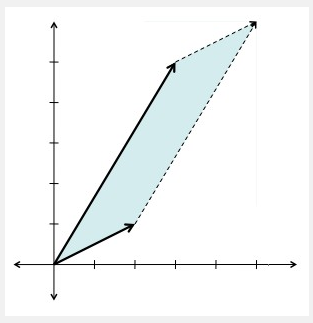
Finding the determinant of the 2 x 2 matrix that describes those two vectors is the same as finding the area of the parallelogram formed by them. Add one more dimension and you get a parallelepiped for your shape and a volume for your determinant.
This has a buttload of applications—like I said, when performing a change of variables when doing multiple integration, but also for finding eigenvalues/eigenvectors and determining whether a set of vectors are linearly independent or not.
I was actually planning on making this a longer blog with an actual calculus application, but a) formatting that would take like 80 years for me and I’ve actually got to study sometime tonight and b) I’ve fallen into the “polar coordinates” article on Wiki and I don’t think I’ll be getting out anytime soon. THEY MAKE ME HAPPY, OKAY?!
Bye.
TWSB: My Initials Stand for a Wallpaper Group
I was screwing around on this site this afternoon and my random scrolling happened to stop on the number 17. Apparently, that’s the number of wallpaper groups.
What’s a wallpaper group?
That’s what I wanted to know.
So I checked it out. Apparently, the wallpaper groups are the 17 possible symmetry groups in the plane. The groups classify patterns based on certain characteristics of symmetry. The Wikipedia page has a bunch of pretty pictures that help show the different symmetries as well as several patterns that fall into each group.
The groups themselves are named with Crystallographic notation. They start with either a p or a c (for primitive cell or face-centered cell, respectively) and then contain several letters or other letters to describe specific components of symmetry (read here!).
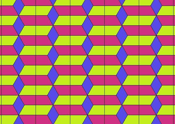
The shorthand name of one of the groups happens to be cmm (my initials!). Patterns with this type of symmetry can be turned upside down (e.g., be rotated 180 degrees) and still look the same. Its lattice is rhombus-shaped. It’s a pretty frequently-encountered pattern, as bricks (like in brick buildings) are often arranged utilizing this group of symmetry.
Here’s a pattern of cmm-type symmetry that I particularly like: