Book Review: Lord of the Flies (Golding)
I done read another one of them books! Here’s Lord of the Flies by William Golding.
Have I read this before: Yup. Way back in 8th grade, though, so it hardly even counts.
Review: I can’t tell if I remembered most of this book or if I just have been able to recognize all the references to it in TV/movies/etc. But I remembered most of this. I think Golding does a really good job of pacing the descent of the boys from “civilized”—having leaders, having tasks, having order—to just completely falling apart and turning against one another. I didn’t remember the ending, though. The ending’s…weird to me.
Favorite part: I enjoyed the escalating loss of control when the hunters would do their “pig killing” reenactments with one another. It seems like a very realistic thing that would happen.
Rating: 6.5/10
Week 9: The Binomial Sign Test for a Single Sample
Today we’re going to look at another nonparametric test: the binomial sign test for a single sample!
When Would You Use It?
The binomial sign test is used in a single sample situation to determine, in a population comprised of two categories, if the proportion of observations in one of the two categories is equal to a specific value.
What Type of Data?
The binomial sign test requires categorical (nominal) data.
Test Assumptions
None listed.
Test Process
Step 1: Formulate the null and alternative hypotheses. The null hypothesis claims that the true proportion of observations in one of the two categories, in the population, is equal to a specific value. The alternative hypothesis claims otherwise (the proportion is either greater than, less than, or not equal to the value claimed in the null hypothesis.
Step 2: Compute the test statistic, a probability value. The test statistic is calculated as follows:

That is, your test statistic is the probability of attaining ≥ r observations from “category 1” in a sample of size n, where r is the number of observations from “category 1” in your original sample.
While you can calculate this value by hand, it may be easier to either use a table or an online calculator.
Step 3: Obtain the p-value. If your alternative hypothesis is non-directional (that is, uses “≠”), your p-value is equal to α/2. If your alternative hypothesis is directional (uses “>” or “<”, your p-value is simply equal to α.
Step 4: Determine your conclusion. This depends on your alternative hypothesis. Let p1 denote the sample proportion of observations falling into “category 1”, and let P denote the test statistic value, as calculated above.
If it is nondirectional (≠) reject H0 if P < α/2.
If the alternative hypothesis is directional (>), reject H0 if p1 > π1 and P < α.
If the alternative hypothesis is directional (<), reject H0 if p1 < π1 and P < α.
Example
For this example, I decided to see if the coin flips from the website Just Flip a Coin were, binomially distributed with π1 = π2 = 0.5. I “flipped” the coin a total of 30 times and recorded my results for “category 1” (heads) and “category 2” (tails). The outcomes are displayed in the table below.
H0: π1 = 0.5
Ha: π1 ≠ 0.5
Set α = 0.05.
Computations:

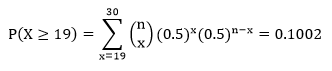
Since P = 0.1002 > 0.025 (α/2 = 0.05/2 = 0.025), we fail to reject H0, the claim that proportion of the number of heads is equal to 0.5 in the population.
Example in R
x = read.table('clipboard', header=F)
pi1= 0.5                                 #hypothesized probability for "heads"
n = length(as.matrix(x))
tab = as.data.frame(table(x))            #observed frequencies
p1 = tab[1,2]
P = 1 - pbinom(p1, size = n, prob = pi1) #test statistic
Anosmia Awareness Day
It’s Anosmia Awareness Day 2016!
I know anosmia isn’t the biggest deal in the world, but there’s a good number of us out there who have it, congenital or otherwise. Here’s a map of just those of us from the Anosmics of the World, Unite! Facebook page who’ve marked our locations for others to see.

Also there’s this, which seems pretty cool.
Anyway.
What’s better than a survey, you ask? A SURVEY ABOUT MY MUSICS
Section 1: Questions About iTunes & Your Songs
How many songs total do you have?: 3,716
How many artists total do you have?: I have no idea. There aren’t a lot of artists for whom I have more than three songs maximum. Maybe 600? 700? No idea.
How many playlists do you have?: 32, haha.
How many music videos do you have (if any)?: 9.
How many TV shows do you have (if any)?: Just 1. All the seasons of Metalocalypse!!
How many podcasts do you have (if any)?: 2. Strong Bad Email (yeah, I know.) and 5 Second Films.
How about books (if any)?: 1 actual book (Leibniz’ Monadology) and 1 audiobook (The Great Gatsby).
How about apps (if any)?: 28, though I only use about 6 or 7 of them frequently.
What is the longest song you have?: New World Symphony by Antonin Dvorak (42:37).
Shortest?: Acoustic Jam by Dethklok (0:28).
Do you use Ping?: No.
Do you use the iTunes Store?: Yup.
How many songs have you purchased from the iTunes store?: Haha. A lot.
Have you recently added an album?: Nope. It’s very rare that I’ll buy an entire album.
Which song has the most plays?: Currently it’s Work This Body by WALK THE MOON.
Do you have a lot of songs you haven’t listened to?: On this computer, yes. I’ve listened to all the songs I own at least once, but I just got this compy in February 2015, and thus have a good number of songs (1,993, to be exact) that haven’t been played yet.
Section 2: Genre Bolding
Bold the genres you have on your iTunes.
Alternative
Blues
Blues-rock
Children’s Music
Christian & Gospel
Classical
Comedy
Country
Dance
Easy Listening
Electronic
Electronica
Folk
Hip Hop
Holiday
House
Indie
Industrial
Instrumental
Jazz
Latino
Metal
Musical
New Age
Pop
Punk
R&B
Rap
Reggae
Rock
Screamo
Soft Rock
Soul
Soundtrack
Techno
Thrash Metal
Trance
World
Section 3: Shuffle
Simply put your iTunes on shuffle, then write the song you get for 20 shuffles
Carry On – Fun.
Candy Shop – 50 Cent and Olivia
Float On – Modest Mouse
Orinoco Flow – Enya
All Star – Smash Mouth
Good Morning Starshine – The 5th Dimension
Bird Dog – The Everley Brothers
Midnight – Coldplay
Without Me – Eminem
I Want Candy – Bow Wow Wow
Trololo (Chiptune Remix) – Robinerd
If We Ever Meet Again – Timbaland
Sleepyhead (Little Vampire Remix) – Passion Pit
Beast – Nico Vega
Possession – Atom and His Package
Caught Up – Usher
Let Me Go – 3 Doors Down
Hook Me Up – The Veronicas
Cupid’s Chokehold – Gym Class Heroes
Atlas – Battles
Section 4: Alphabet – Artists
Name an artist you have for each letter/number.
A: Apocalyptica
B: Barenaked Ladies
C: Cut Copy
D: Deep Forest
E: The Everly Brothers
F: Fleet Foxes
G: The Guggenheim Grotto
H: Hot Chip
I: Imogen Heap
J: James Horner
K: The Killers
L: Lady Gaga
M: Miike Snow
N: Neil Diamond
O: OK Go
P: Pony Pony Run Run
Q: Queens of the Stone Age
R: Robyn
S: Sugar Ray
T: TNGHT
U: Usher
V: The Veronicas
W: WALK THE MOON
X: XTC
Y: Yngwie Malmsteen
Z: Zeds Dead
#: The 1975
Section 5: Top 25 Most Played
List your Top 25 most played songs.
Work This Body – WALK THE MOON
Doin’ It Right (feat. Panda Bear) – Daft Punk
Jealous (I Ain’t With It) – Chromeo
Say What You Want – Barenaked Ladies
Over My Head (Gabe Flaherty Remix) – The Fray
Gold (Thomas Jack Radio Edit) – Gabriel Rios
This Is So Good – Ehrencrona|
Pieces of Me – Ashlee Simpson
Good Life – OneRepublic
Lone Digger – Caravan Palace
Call on Me – Eric Prydz
Get Over It – OK Go
Doin’ It Right (Decadon Remix) – Daft Punk
Did I Say That Out Loud – Barenaked Ladies
I Won’t Let You Down – OK Go
Amazon – Gabe Flaherty
Sleepyhead – Passion Pit
Dare You to Move – Vitamin String Quartet
Pumped Up Kicks (Gabe Flaherty Remix) – Foster the People
Sleepyhead (Jazzsteppa Remix) – Passion Pit
Take a Walk (A Capella) – Passion Pit
Madness – Muse
Suit & Tie (Oliver Nelson Remix) – Justin Timberlake
Mirrors (Radio Edit) – Justin Timberlake
Sleepyhead (Cillo Remix) – Passion Pit
Foods’n’things
Do y’all want some more recipes?
OF COURSE YOU DO!
(I’m ignoring the crappy parts of my life by using the internet. Is it working?)
(I also don’t know how many of these I’ve previously posted on here, so apologies in advance for any duplicates.)
One Pan Roasted Chicken and Veggies
Perfect Steakhouse Baked Potato
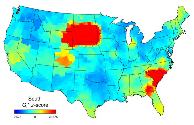
Word Mapper
It lets you type in a word (I think it only has the most frequently used 100,000 words, though?) and will map its frequency of use in tweets (either by county or just by hotspots) across the continental US.
Here are some fun ones.
The differing distributions of “geek”, “dork”, and “nerd”:


“Canada”, “Mexico”, and “America” (I would have used “United States”, but it just takes words, not phrases):


“North” and “south” are nicely clustered around the states with those words in their names:

Idaho!

I’m a-feared
UGH THE TEST IS OVER. Thank god.
It wasn’t awful, but I know I made at least one—maybe two—stupid little mistakes. I’m hoping Dr. Lu will be merciful and see that I do understand what I’m doing, I just made dumb math errors.
‘Cause that’s what I do.
Now it’s time to do nothing school-related for the rest of the day.
Week 8: The Chi-Square Goodness-of-Fit Test
Today we’re continuing the theme of nonparametric tests with the chi-square goodness-of-fit test!
When Would You Use It?
The chi-square goodness-of-fit test is a nonparametric test used in a single sample situation to determine if a sample originates from a population for which the observed cell (category) frequencies different from the expected cell (category) frequencies. Basically, this test is used when a particular “distribution” is expected of the categories of a variable and a researcher wants to know if that distribution fits the data.
What Type of Data?
The chi-square goodness-of-fit test requires categorical (nominal) data.
Test Assumptions
- Categorical or nominal data are used in the analysis (the data should represent frequencies for mutually exclusive categories).
- The data consist of a random sample of n observations.
- The expected frequency (as calculated below) of each cell is 5 or greater.
Test Process
Step 1: Formulate the null and alternative hypotheses. The null hypothesis claims that the observed frequency of each cell is equal to the expected frequency of that cell, while the alternative hypothesis claims that at least one cell has an observed frequency that differs from the expected frequency.
Step 2: Compute the test statistic, a chi-square value. The calculations are as follows:
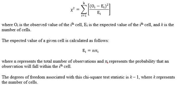
Step 3: Obtain the p-value associated with the calculated chi-square. The p-value indicates the probability of observing deviations from the expected values that are larger than those in the observed sample, under the assumption that the null hypothesis is true.
Step 4: Determine the conclusion. If the p-value is larger than the prespecified α-level, fail to reject the null hypothesis (that is, retain the claim that the observed frequencies in the cells are equal to the expected frequencies of the cells). If the p-value is smaller than the prespecified α-level, reject the null hypothesis in favor of the alternative.
Example
For this test’s example, I wanted to determine if the dice on my iPod Yahtzee app were fair. That is, I wanted to see if there was an equal probability for all six sides to come up on any given roll. So I rolled the five dice 115 times (for a total of n = 575 individual die rolls) and simply recorded the faces showing (note that I did not actually “play” Yahtzee while doing this, which is to say that I just kept rolling all five dice no matter what happened and I didn’t “hold” any of them at any point). I’m going to claim in my null hypothesis that all six side values have an equal probability of showing on a given die. That is,
H0: p1 = p2 = p3 = p4 = p5 = p6 = 1/6
Ha: The probability for at least one value is not 1/6
Set α = 0.05.
Computations:

Since our p-value is larger than our alpha level of .05, we fail to reject H0 and claim that the observed values are equal to the expected values and the dice are fair.
Example in R
x=read.table('clipboard', header=F)
n=length(x)
tab=as.data.frame(table(x))           #observed frequencies
p=1/length(tab$x)
Chi=rep(NaN,length(tab$x))
for (i in 1:length(tab$x)){
Chi[i]=((tab$Freq[i]-(p*n))^2)/(p*n)
}
Chisquare=sum(Chi)
1-pchisq(Chisquare,length(tab$x)-1)   #p-value
Have an Art that’s Not a Heart!
SHOCKING

Sorry I keep posting about school. (I’m not sorry at all.)
This video accurately depicts the change in my attitude and approach to grad school, pre- and post-February 2nd.
The day you identify with a HowToBasic video is the day you know that things have gone horribly wrong.
This Week’s Science Blog: Remember When I Used to do a Weekly Science Blog?
SUN NEWS!
According to research at the University of Warwick, the sun may have the potential to superflare. What’s a superflare? It’s supercool. Superflares are like solar flares, only thousands of times more powerful. According to the lead researcher at Warwick, Chloe Pugh, if the sun were to superflare, pretty much all of earth’s communications and energy systems could fail. Radio signals disabled, huge blackouts, all that fun stuff. But according to Pugh, the conditions needed for a superflare are extremely unlikely to occur on the sun.
But how did they actually figure out that it is possible for the sun to superflare? Using NASA’s Kepler space telescope, the researchers found a binary star, KIC9655129, which has been shown to superflare. The researchers suggest that due to the similarities between the sun’s solar flares and the superflares of KIC9655129, the underlying physics of both phenomena may be the same.
Cool!
Week 7: The Kolmogorov-Smirnov Goodness-of-Fit Test for a Single Sample
Today we’re going to do our first test of goodness-of-fit with the Kolmogorov-Smirnov goodness-of-fit test for a single sample.
When Would You Use It?
The Kolmogorov-Smirnov goodness-of-fit test is a nonparametric test used in a single sample situation to determine if the distribution of a sample of values conforms to a specific population (or probability) distribution.
What Type of Data?
The Kolmogorov-Smirnov goodness-of-fit test requires ordinal data.
Test Assumptions
None listed.
Test Process
Step 1: Formulate the null and alternative hypotheses. The null hypothesis claims that the distribution of the data in the sample is consistent with the hypothesized theoretical population distribution. The alternative claims that the distribution of the data in the sample is inconsistent with the hypothesized theoretical population distribution.
Step 2: Compute the test statistic. The test statistic, in the case of this test, is defined by the point that represents the greatest vertical distance at any point between the cumulative probability distribution constructed from the sample and the cumulative probability distribution constructed under the hypothesized population distribution. Since the specifics of the cumulative probability distribution calculations depend on which distributions are used, I will refer you to the example shown below to show how these calculations are done in a specific testing situation.
Step 3: Obtain the critical value. Unlike most of the tests we’ve done so far, you don’t get a precise p-value when computing the results here. Rather, you calculate your test statistic and then compare it to a specific value. This is done using a table (such as the one here). Find the number at the intersection of your sample size n and the specified alpha-level. Compare this value with your test statistic.
Step 4: Determine the conclusion. If your test statistic is equal to or larger than the table value, reject the null hypothesis (that is, claim that the distribution of the data is inconsistent with the hypothesized population distribution). If your test statistic is less than the table value, fail to reject the null.
Example
For this test’s example, I wanted to determine, from a sample of n = 59 IQ scores, if scores in the population follow a normal distribution with a mean µ = 100 and standard deviation σ = 15. Set α = 0.05.
H0: IQ scores in the population follow a normal distribution with a mean of 100 and a standard deviation of 15.
Ha: IQ scores in the population deviate from a normal distribution with a mean of 100 and a standard deviation of 15.
Computations:
For the computations section of this test, I will display a table of values for the first three and the last of the IQ scores (sorted from smallest to largest) and describe what the values are and how the test statistic is obtained.

Column A represents the IQ scores of the sample, ranked from lowest to highest.
Column B represents the z-scores of the IQ tests, calculated by taking the difference of the score and the mean (100), then dividing by the standard deviation (15).
Column B is not necessary, but is used to make the calculation of Column C easier. Column C is the proportion of cases between the z-score (Column B) and the hypothesized mean of the population’s distribution (100 in this case). For example, for an IQ of 81, the proportion of scores falling between 82 and 100 is .385.
Column D represents the percentile rank of a given IQ score in the hypothesized population distribution. An IQ of 82, for example, is the 11.5th percentile.
Column E represents the cumulative proportion, in the sample, for each IQ. For an IQ of 82, the cumulative proportion is just 1/59, while the cumulative proportion for the highest value, 145, is 59/59.
Column F is the absolute difference between the ith values in Column D and Column E. This represents the differences between the proportions in the sample population and the proportions expected under the hypothesized population distribution.
Finally, Column G is the absolute difference between the value of Column D for a given row and the value of Column E for the preceeding row. For example, for an IQ of 89, Column G is calculated by taking |0.232 – 0.017|.
The test statistic is obtained by determining the largest value from either Column F or Column G. That is, whichever column has the largest value, then that largest value becomes the test statistic. When these values are computed for the whole dataset, the largest value is 0.438. This value is compared to the critical value at α = 0.05, n > 35, which ends up being:

Since our test statistic is larger than our critical value, we reject H0 and claim that IQ scores in the population deviate from a normal distribution with mean 100 and standard deviation 15.
Example in R
x=read.table('clipboard', header=F)
x=as.matrix(x)
x=sort(x)                                                   #column A
mu=100
sd=15
B=(x-mu)/sd                                                 #column B
pmu=.5
pz=pnorm(abs(z), mean = 0, sd = 1, lower.tail = TRUE)
C=abs(pmu-pz) #column C
D=pnorm(z, mean = 0, sd = 1, lower.tail = TRUE)             #column D
E=rep(NaN,length(x))                                        #column E
for (i in 1:length(x)){
e[i]=i/length(x)
}
F=abs(e-dz)                                                 #column F
ee=c(0,e[1:(length(x)-1)])
G=abs(ee-dz)                                                #column G
if(max(G)>max(F)){Tstat=max(G)}else{Tstat=max(F)}
Tstat                                                       #test statistic
Go? OK!
So remember this post when I said that OK Go’s next step in the world of music videos would be to shoot one in space?
Well, I was close.
Zero gravity! Very cool.
Apparently there was lots of throwing up while filming this, haha.
This Just In: People Suck at Walking
Walking.
For something so natural for humans to do, we sure do suck at it.
The thing that really pisses me off is when you’ve got some slow little fart in front of you who decides that he needs to walk RIGHT IN THE CENTER OF THE DAMN SIDEWALK and is completely oblivious (usually due to a phone) to everything around him.
Like, I’m making all sorts of noise behind the guy to warn him that he’s not the only one on the sidewalk and is certainly not one of the faster ones, and he’s just “duurrrrr smart phone.”
Then I end up finally having to walk off the side of the sidewalk to pass him, and he gives me the dirtiest little “how dare you” look.
Dude. Seriously. It’s not my fault you’re an idiot. MOVE TO THE SIDE OF THE SIDEWALK IF YOU’RE GOING TO WALK AT THE PACE OF A COMATOSE SNAIL.
NNNNNNNNNNNNNNGH.
This is how I feel when I go to pass these types of walkers.

(Yes, I made a .gif from that YouTube video. It’s pretty much my favorite video ever.)
Rage Quit
So thanks to Nate listening to the playlist of Michael’s Rage Quit on YouTube, I’ve been listening to my favorite old Rage Quits all day at school. So I’ll put them all here, ‘cause even though I’ve mentioned most (all?) of these in my blog at some point, it’s nice to have everything together. And I haven’t mentioned any Rage Quits in a while.
These are vaguely ranked.
The Impossible Game Level Pack: Level 2
The Impossible Game Level Pack: Level 3
Realistic Summer Sports Simulator
UUUUUUUUUUUUUUUUUUUGH.
Have some gifs n’ stuff, ‘cause I’m freaking done with life right now.


Week 6: The Wilcoxon Signed-Ranks Test
Today we’re going to talk about our first nonparametric test: the Wilcoxon signed-ranks test!
When Would You Use It?
The Wilcoxon signed-ranks test is a nonparametric test used in a single sample situation to determine if the sample originates from a population with a specific median θ.
What Type of Data?
The Wilcoxon signed-ranks test requires ordinal data.
Test Assumptions
- The sample is a simple random sample from the population of interest.
- The original scores obtained for each of the individuals in the sample are in the format of interval or ratio data.
- The underlying population distribution is symmetrical.
Test Process
Step 1: Formulate the null and alternative hypotheses. The null hypothesis claims that the median in the population is equal to a specific value; the alternative hypothesis claims otherwise (the population median is greater than, less than, or not equal to the value specified in the null hypothesis).
Step 2: Compute the test statistic. Since this is best done with data, please see the example shown below to see how this is done.
Step 3: Obtain the critical value. Unlike most of the tests we’ve done so far, you don’t get a precise p-value when computing the results here. Rather, you calculate your test statistic and then compare it to a specific value. This is done using a table (such as the one here). Find the number at the intersection of your sample size n and the specified alpha-level. Compare this value with your test statistic.
Step 4: Determine the conclusion. If your test statistic is equal to or less than the table value, reject the null hypothesis. If your test statistic is greater than the table value, fail to reject the null (that is, claim that the median in the population is in fact equal to the value specified in the null hypothesis).
Example
The data for this example come from a little analysis of my Facebook friends’ birthdays I did awhile ago. In that analysis, I recorded the birth months for the n = 97 friends who had their birthdays visible. All I did at the time was see how many birthdays there were per month. Now, however, I want to see if the median number of birthdays per month is equal to a certain value—say, 8. Set α = 0.05.
H0: θ = 8
Ha: θ ≠ 8
The following table shows several different columns of information. I will explain the columns below.

Column 1 is just the name of the month.
Column 2 is the number of observed birthdays in my sample for that corresponding month.
Column 3 is calculated by taking the number of observed birthdays minus the hypothesized median, which is θ = 8 in this case.
Column 4 is the absolute value of the difference in Column 3.
Column 5 is the rank of the value in Column 4. Ranking is done as follows: rank the values of Column 4 from smallest to largest. If there are ties, sum the number of ranks that are taken by the ties, and then divide that value by the number of ties. For example, there are five months that have a |D| = 3. That means that this tied value takes up the rank places of the 1st, 2nd, 3rd, 4th, and 5th observations, had they not been all tied at 1. Thus, I sum these rank places and divide by 5 to get (1+2+3+4+5)/5 = 3, then assign all these five months the rank of 3.
Column 6 contains the same values as Column 5, but signs them depending on the sign in Column 3.
The next step is to sum all the positive ranks in Column 6 and sum all the negative ranks in Column 6. Doing so, we get:
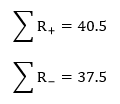
The test statistic itself is the absolute value of the smaller of the above values; in this case, we get T = 37.5. In the table, the critical value for n = 12 and α = 0.05 for a two-tailed test is 13. Since T > 13, we fail to reject the null and retain the claim that the population median is, in fact, 8.
Example in R
No R example this week; most of this is easy enough to do by hand for a small-ish sample.
In a time of chimpanzees, I was a robot
A lot of these are great.
That’s all I have to say today, sorry.
*angry huffing*
So this week has been awful.
But luckily I have a ridiculously incredible fiancé who picked up some super colorful flowers for me on his way home from work today, just because he knows things have gone south for me over the past few days and he wanted to show he cares.
I can’t wait to marry this man.
Two other completely unrelated bits of news:
- I had a scintillating scotoma migraine this morning. It’s been awhile since I’ve had one of those.
- I want you all to hear 2016’s first five-star song. It’s incredible.

