Week 13: F Test for Two Population Variances
Today we’re going to talk about variances. Specifically, the F test for two population variances!
When Would You Use It?
The F test for two population variances is a parametric test used to determine if two independent samples represent two populations with homogeneous (similar) variances.
What Type of Data?
The F test for two population variances requires interval or ratio data.
Test Assumptions
None listed.
Test Process
Step 1: Formulate the null and alternative hypotheses. The null hypothesis claims that the two population variances are equal. The alternative hypothesis claims otherwise (one population variance is greater than the other, less than the other, or that the variances are simply not equal).
Step 2: Compute the test statistic, an F value. The test statistic is computed as follows:

Step 3: Obtain the p-value associated with the calculated F value. The p-value indicates the probability of a difference in the two sample variances that is equal to or more extreme than the observed difference between the sample variances, under the assumption that the null hypothesis is true. The two degrees of freedom associated with the F value are df1 = n1-1 and df2 = n2-1, where n1 and n2 are the respective sample sizes of the first and second sample.
Step 4: Determine the conclusion. If the p-value is larger than the prespecified α-level, fail to reject the null hypothesis (that is, retain the claim that the population means are equal). If the p-value is smaller than the prespecified α-level, reject the null hypothesis in favor of the alternative.
Example
The data for this example come from my walking data from 2013 and 2015. I want to see if there is a significant difference in the mileage variance for these two years (in other words, was I less consistent with the length of my walks in one year versus the other? Set α = 0.05.
H0: σ12 = σ22 (or σ12 – σ22 = 0)
Ha: σ12 ≠ σ22 (or σ12 – σ22 ≠ 0)
Computations:

Since our p-value is smaller than our alpha-level, we reject H0 and claim that the population variances are significantly different (with evidence in favor of the variance being higher for 2015).
Example in R
year2013=read.table('clipboard', header=F) #data from 2013
year2015=read.table('clipboard', header=F) #data from 2015
s1=var(year2013)
s2=var(year2015)
df1=length(year2013)-1
df2=length(year2015)-1
F=s2/s1                        #test statistic
pval = (1-pf(F, df2, df1))     #p-value
Week 12: The t Test for Two Independent Samples
Today we’re going to talk about our first test involving two samples: the t test for two independent samples!
When Would You Use It?
The t test for two independent samples is a parametric test used to determine if two independent samples represent two populations with different mean values.
What Type of Data?
The t test for two independent samples requires interval or ratio data.
Test Assumptions
- Each sample is a simple random sample from the populations they represent.
- The distributions underlying each of the populations are normal.
- The variances of the underlying populations are equal (homogeneity of variance; a formal test for this will come in a later week).
Test Process
Step 1: Formulate the null and alternative hypotheses. The null hypothesis claims that the two sample means are equal. The alternative hypothesis claims otherwise (one population mean is greater than the other, less than the other, or that the means are simply not equal).
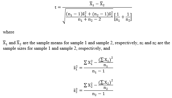
Step 2: Compute the t-score. The t-score is computed as follows:
Step 3: Obtain the p-value associated with the calculated t-score. The p-value indicates the probability of a difference in the two sample means that is equal to or more extreme than the observed difference between the sample means, under the assumption that the null hypothesis is true.
Step 4: Determine the conclusion. If the p-value is larger than the prespecified α-level, fail to reject the null hypothesis (that is, retain the claim that the population means are equal). If the p-value is smaller than the prespecified α-level, reject the null hypothesis in favor of the alternative.
Example
The data for this example come from the midterm scores of my lab section for STAT 213. While lab attendance is technically optional, the students’ attendance is recorded for each lab (if they show up to lab, they basically get additional instructional materials unlocked to help them study more).
I wanted to see if there was a significant difference in the average midterm score for students who attended lab at least half the time (sample 1) and students who attended lab less than half the time (sample 2). Specifically, I wanted to test the claim that attending lab more frequently was associated with a higher midterm score. Here, n1 = 17 and n2 = 13. Set α = 0.05.
H0: µ1 = µ2 (or µ1 – µ2 = 0)
Ha: µ1 > µ2 (or µ1 – µ2 > 0)
Computations:

Since our p-value is smaller than our alpha-level, we reject H0 and claim that the population means are significantly different (with evidence in favor of the mean being higher for those attending labs more often).
Example in R
x=read.table('clipboard', header=T)
attach(x)
x1=subset(x,attended==1)[,1]                 #attended lab
x2=subset(x,attended==0)[,1]                 #did not attend lab
n1=length(x1)
n2=length(x2)
xbar1=mean(x1)
xbar2=mean(x2)
s1=((sum(x1^2)-(((sum(x1))^2)/n1))/(n1-1))
s2=((sum(x2^2)-(((sum(x2))^2)/n2))/(n2-1))
t = (xbar1 - xbar2)/sqrt(((((n1-1)*s1)
    +((n2-1)*s2))/(n1+n2-2))*((1/n1)+(1/n2))) #test statistic
pval = (1-pt(t, n-1))                         #p-value
Week 11: The Single-Sample Runs Test
Today we’re going to look at another nonparametric test: the single-sample runs test.
When Would You Use It?
The runs test is a nonparametric test used in a single sample situation to determine if the distribution of a series of binary events, in the population, is random.
What Type of Data?
The single sample runs test requires categorical (nominal) data.
Test Assumptions
None listed.
Test Process|
Step 1: Formulate the null and alternative hypotheses. The null hypothesis claims that the events in the underlying population (represented by the sample series) are distributed randomly. The alternative hypothesis claims that the events in the underlying population are distributed nonrandomly.
Step 2: Compute the number of times each of the two alternatives appears in the sample series (n1 and n2) and the number of runs, r, in the series. A run is a sequence within the series in which one of the alternatives occurs on consecutive trials.
Step 3: Obtain the critical value. Unlike most of the tests we’ve done so far, you don’t get a precise p-value when computing the runs test results. Rather, you calculate your r and then compare it to an upper and lower limit for your specific n1 and n2 values. This is done using a table (such as the one here*). For the values of n1 and n2 in your sample (labeled on this table as n and m), find the intersecting cell of the two values.
Step 4: Determine the conclusion. If your r is greater than or equal to the larger number or smaller than or equal to the smaller number in that cell, you have a statistically significant result, meaning you reject the null (that is, reject the claim that the distribution of the binary events in the population is nonrandom). If your r is between the smaller and larger number, fail to reject the null.
Example
For this example, I decided to see if the coin flips from the website Just Flip a Coin were, in fact, random. I “flipped” the coin a total of 30 times and recorded my results as “H” for heads and “T” for tails. This series is recorded below.
H0: The distribution of heads and tails in the population is random
Ha: The distribution of heads and tails in the population is nonrandom.
THTTHHHHHHTHTTHHTTHHTHHHTHHHHT
Computations:
T H TT HHHHHH T H TT HH TT HH T HHH T HHHH T
n1 = 19 (heads)
n2 = 11 (tails)
r = 15
According to the table, my lower bound is 9 and my upper bound is 21. Since my r is in between these two values, I do not have a statistically significant result. I fail to reject H0 and claim that the distribution of heads and tails in the population is indeed random.
*Note that this table, like many others, only has a maximum of 20 for either n or m, and is constructed with α = 0.05 for the two-sided test and α = 0.025 for the one-sided test.
Example in R
No R example this week, since it’s probably more work to do this in R than it is to do it by hand, haha.
Week 10: The z Test for a Population Proportion
Today it’s time for yet another test: the z test for a population proportion!
When Would You Use It?
The z test for a population proportion is used to determine if, in an underlying population comprised of two categories, the proportion of observations (in a sample) in one of the two categories is equal to a specific value.
What Type of Data?
The z test for a population proportion requires categorical (nominal) data.
Test Assumptions
- Each of the n independent observations is randomly selected from a population, and each observation can be classified into one of two mutually exclusive categories.
- It is recommended that this test is employed when the sample is not too small (n > 11).
Test Process
Step 1: Formulate the null and alternative hypotheses. The null hypothesis claims that the likelihood an observation will fall into Category 1 in the population is equal to a certain probability. The alternative hypothesis claims otherwise (that the population proportion for Category 1 is not equal to the value stated in the null).
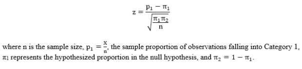
Step 2: Compute the test statistic, a z-score. The test statistic is computed as follows:
Step 3: Obtain the p-value associated with the calculated z-score. The p-value indicates the probability of observing a sample proportion as extreme or more extreme than the observed sample proportion, under the assumption that the null hypothesis is true.
Step 4: Determine the conclusion. If the p-value is larger than the prespecified α-level, fail to reject the null hypothesis (that is, retain the claim that the probability of falling into Category 1 in the population is equal to the value specified in the null hypothesis). If the p-value is smaller than the prespecified α-level, reject the null hypothesis in favor of the alternative.
Example
The data for this example come from my n = 30 students from one of my STAT 213 labs. I want to test the hypothesis, based on my lab, that the proportion of students who come to lab for ALL the 213 labs (for this particular instructor) is 40%. We take attendance, so we know who’s there and who’s not for a given week (note, however, that I’m going to randomly select an attendance sheet from one of the weeks of lab, AND I actually never pay attention to what the proportion of students who show up is, so I’m really just guessing about 40%). So let’s do it! Set α = 0.05 and let π denote the proportion of individuals to come to lab.
H0: π = .4
Ha: π ≠ .4
Computations:

Since our p-value is (only slightly) larger than our alpha-level, we fail to reject H0 and claim that the population proportion of students who attend labs is, in fact, .4.
Example in R
dat = read.table('clipboard',header=F) #'dat' is the name of the imported raw data
                                       #'dat' coded such that 0 = did not attend, 1 = attended
n = nrow(dat)
X = sum(dat)
p1 =  X/n
pi1 = .4
z = (p1-pi1)/(sqrt((pi1*(1-pi1))/n))  #z-score
pval = (1-pnorm(z))*2                 #p-value
                                      #pnorm calculates the left-hand area
                                      #multiply by two because it is a two-sided test
Week 9: The Binomial Sign Test for a Single Sample
Today we’re going to look at another nonparametric test: the binomial sign test for a single sample!
When Would You Use It?
The binomial sign test is used in a single sample situation to determine, in a population comprised of two categories, if the proportion of observations in one of the two categories is equal to a specific value.
What Type of Data?
The binomial sign test requires categorical (nominal) data.
Test Assumptions
None listed.
Test Process
Step 1: Formulate the null and alternative hypotheses. The null hypothesis claims that the true proportion of observations in one of the two categories, in the population, is equal to a specific value. The alternative hypothesis claims otherwise (the proportion is either greater than, less than, or not equal to the value claimed in the null hypothesis.
Step 2: Compute the test statistic, a probability value. The test statistic is calculated as follows:

That is, your test statistic is the probability of attaining ≥ r observations from “category 1” in a sample of size n, where r is the number of observations from “category 1” in your original sample.
While you can calculate this value by hand, it may be easier to either use a table or an online calculator.
Step 3: Obtain the p-value. If your alternative hypothesis is non-directional (that is, uses “≠”), your p-value is equal to α/2. If your alternative hypothesis is directional (uses “>” or “<”, your p-value is simply equal to α.
Step 4: Determine your conclusion. This depends on your alternative hypothesis. Let p1 denote the sample proportion of observations falling into “category 1”, and let P denote the test statistic value, as calculated above.
If it is nondirectional (≠) reject H0 if P < α/2.
If the alternative hypothesis is directional (>), reject H0 if p1 > π1 and P < α.
If the alternative hypothesis is directional (<), reject H0 if p1 < π1 and P < α.
Example
For this example, I decided to see if the coin flips from the website Just Flip a Coin were, binomially distributed with π1 = π2 = 0.5. I “flipped” the coin a total of 30 times and recorded my results for “category 1” (heads) and “category 2” (tails). The outcomes are displayed in the table below.
H0: π1 = 0.5
Ha: π1 ≠ 0.5
Set α = 0.05.
Computations:

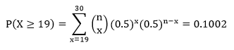
Since P = 0.1002 > 0.025 (α/2 = 0.05/2 = 0.025), we fail to reject H0, the claim that proportion of the number of heads is equal to 0.5 in the population.
Example in R
x = read.table('clipboard', header=F)
pi1= 0.5                                 #hypothesized probability for "heads"
n = length(as.matrix(x))
tab = as.data.frame(table(x))            #observed frequencies
p1 = tab[1,2]
P = 1 - pbinom(p1, size = n, prob = pi1) #test statistic
Week 8: The Chi-Square Goodness-of-Fit Test
Today we’re continuing the theme of nonparametric tests with the chi-square goodness-of-fit test!
When Would You Use It?
The chi-square goodness-of-fit test is a nonparametric test used in a single sample situation to determine if a sample originates from a population for which the observed cell (category) frequencies different from the expected cell (category) frequencies. Basically, this test is used when a particular “distribution” is expected of the categories of a variable and a researcher wants to know if that distribution fits the data.
What Type of Data?
The chi-square goodness-of-fit test requires categorical (nominal) data.
Test Assumptions
- Categorical or nominal data are used in the analysis (the data should represent frequencies for mutually exclusive categories).
- The data consist of a random sample of n observations.
- The expected frequency (as calculated below) of each cell is 5 or greater.
Test Process
Step 1: Formulate the null and alternative hypotheses. The null hypothesis claims that the observed frequency of each cell is equal to the expected frequency of that cell, while the alternative hypothesis claims that at least one cell has an observed frequency that differs from the expected frequency.
Step 2: Compute the test statistic, a chi-square value. The calculations are as follows:
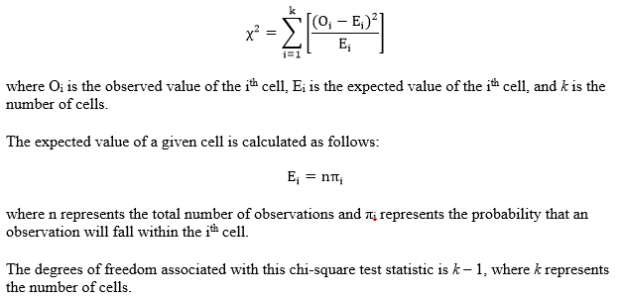
Step 3: Obtain the p-value associated with the calculated chi-square. The p-value indicates the probability of observing deviations from the expected values that are larger than those in the observed sample, under the assumption that the null hypothesis is true.
Step 4: Determine the conclusion. If the p-value is larger than the prespecified α-level, fail to reject the null hypothesis (that is, retain the claim that the observed frequencies in the cells are equal to the expected frequencies of the cells). If the p-value is smaller than the prespecified α-level, reject the null hypothesis in favor of the alternative.
Example
For this test’s example, I wanted to determine if the dice on my iPod Yahtzee app were fair. That is, I wanted to see if there was an equal probability for all six sides to come up on any given roll. So I rolled the five dice 115 times (for a total of n = 575 individual die rolls) and simply recorded the faces showing (note that I did not actually “play” Yahtzee while doing this, which is to say that I just kept rolling all five dice no matter what happened and I didn’t “hold” any of them at any point). I’m going to claim in my null hypothesis that all six side values have an equal probability of showing on a given die. That is,
H0: p1 = p2 = p3 = p4 = p5 = p6 = 1/6
Ha: The probability for at least one value is not 1/6
Set α = 0.05.
Computations:

Since our p-value is larger than our alpha level of .05, we fail to reject H0 and claim that the observed values are equal to the expected values and the dice are fair.
Example in R
x=read.table('clipboard', header=F)
n=length(x)
tab=as.data.frame(table(x))           #observed frequencies
p=1/length(tab$x)
Chi=rep(NaN,length(tab$x))
for (i in 1:length(tab$x)){
Chi[i]=((tab$Freq[i]-(p*n))^2)/(p*n)
}
Chisquare=sum(Chi)
1-pchisq(Chisquare,length(tab$x)-1)   #p-value
Week 7: The Kolmogorov-Smirnov Goodness-of-Fit Test for a Single Sample
Today we’re going to do our first test of goodness-of-fit with the Kolmogorov-Smirnov goodness-of-fit test for a single sample.
When Would You Use It?
The Kolmogorov-Smirnov goodness-of-fit test is a nonparametric test used in a single sample situation to determine if the distribution of a sample of values conforms to a specific population (or probability) distribution.
What Type of Data?
The Kolmogorov-Smirnov goodness-of-fit test requires ordinal data.
Test Assumptions
None listed.
Test Process
Step 1: Formulate the null and alternative hypotheses. The null hypothesis claims that the distribution of the data in the sample is consistent with the hypothesized theoretical population distribution. The alternative claims that the distribution of the data in the sample is inconsistent with the hypothesized theoretical population distribution.
Step 2: Compute the test statistic. The test statistic, in the case of this test, is defined by the point that represents the greatest vertical distance at any point between the cumulative probability distribution constructed from the sample and the cumulative probability distribution constructed under the hypothesized population distribution. Since the specifics of the cumulative probability distribution calculations depend on which distributions are used, I will refer you to the example shown below to show how these calculations are done in a specific testing situation.
Step 3: Obtain the critical value. Unlike most of the tests we’ve done so far, you don’t get a precise p-value when computing the results here. Rather, you calculate your test statistic and then compare it to a specific value. This is done using a table (such as the one here). Find the number at the intersection of your sample size n and the specified alpha-level. Compare this value with your test statistic.
Step 4: Determine the conclusion. If your test statistic is equal to or larger than the table value, reject the null hypothesis (that is, claim that the distribution of the data is inconsistent with the hypothesized population distribution). If your test statistic is less than the table value, fail to reject the null.
Example
For this test’s example, I wanted to determine, from a sample of n = 59 IQ scores, if scores in the population follow a normal distribution with a mean µ = 100 and standard deviation σ = 15. Set α = 0.05.
H0: IQ scores in the population follow a normal distribution with a mean of 100 and a standard deviation of 15.
Ha: IQ scores in the population deviate from a normal distribution with a mean of 100 and a standard deviation of 15.
Computations:
For the computations section of this test, I will display a table of values for the first three and the last of the IQ scores (sorted from smallest to largest) and describe what the values are and how the test statistic is obtained.

Column A represents the IQ scores of the sample, ranked from lowest to highest.
Column B represents the z-scores of the IQ tests, calculated by taking the difference of the score and the mean (100), then dividing by the standard deviation (15).
Column B is not necessary, but is used to make the calculation of Column C easier. Column C is the proportion of cases between the z-score (Column B) and the hypothesized mean of the population’s distribution (100 in this case). For example, for an IQ of 81, the proportion of scores falling between 82 and 100 is .385.
Column D represents the percentile rank of a given IQ score in the hypothesized population distribution. An IQ of 82, for example, is the 11.5th percentile.
Column E represents the cumulative proportion, in the sample, for each IQ. For an IQ of 82, the cumulative proportion is just 1/59, while the cumulative proportion for the highest value, 145, is 59/59.
Column F is the absolute difference between the ith values in Column D and Column E. This represents the differences between the proportions in the sample population and the proportions expected under the hypothesized population distribution.
Finally, Column G is the absolute difference between the value of Column D for a given row and the value of Column E for the preceeding row. For example, for an IQ of 89, Column G is calculated by taking |0.232 – 0.017|.
The test statistic is obtained by determining the largest value from either Column F or Column G. That is, whichever column has the largest value, then that largest value becomes the test statistic. When these values are computed for the whole dataset, the largest value is 0.438. This value is compared to the critical value at α = 0.05, n > 35, which ends up being:

Since our test statistic is larger than our critical value, we reject H0 and claim that IQ scores in the population deviate from a normal distribution with mean 100 and standard deviation 15.
Example in R
x=read.table('clipboard', header=F)
x=as.matrix(x)
x=sort(x)                                                   #column A
mu=100
sd=15
B=(x-mu)/sd                                                 #column B
pmu=.5
pz=pnorm(abs(z), mean = 0, sd = 1, lower.tail = TRUE)
C=abs(pmu-pz) #column C
D=pnorm(z, mean = 0, sd = 1, lower.tail = TRUE)             #column D
E=rep(NaN,length(x))                                        #column E
for (i in 1:length(x)){
e[i]=i/length(x)
}
F=abs(e-dz)                                                 #column F
ee=c(0,e[1:(length(x)-1)])
G=abs(ee-dz)                                                #column G
if(max(G)>max(F)){Tstat=max(G)}else{Tstat=max(F)}
Tstat                                                       #test statistic
Week 6: The Wilcoxon Signed-Ranks Test
Today we’re going to talk about our first nonparametric test: the Wilcoxon signed-ranks test!
When Would You Use It?
The Wilcoxon signed-ranks test is a nonparametric test used in a single sample situation to determine if the sample originates from a population with a specific median θ.
What Type of Data?
The Wilcoxon signed-ranks test requires ordinal data.
Test Assumptions
- The sample is a simple random sample from the population of interest.
- The original scores obtained for each of the individuals in the sample are in the format of interval or ratio data.
- The underlying population distribution is symmetrical.
Test Process
Step 1: Formulate the null and alternative hypotheses. The null hypothesis claims that the median in the population is equal to a specific value; the alternative hypothesis claims otherwise (the population median is greater than, less than, or not equal to the value specified in the null hypothesis).
Step 2: Compute the test statistic. Since this is best done with data, please see the example shown below to see how this is done.
Step 3: Obtain the critical value. Unlike most of the tests we’ve done so far, you don’t get a precise p-value when computing the results here. Rather, you calculate your test statistic and then compare it to a specific value. This is done using a table (such as the one here). Find the number at the intersection of your sample size n and the specified alpha-level. Compare this value with your test statistic.
Step 4: Determine the conclusion. If your test statistic is equal to or less than the table value, reject the null hypothesis. If your test statistic is greater than the table value, fail to reject the null (that is, claim that the median in the population is in fact equal to the value specified in the null hypothesis).
Example
The data for this example come from a little analysis of my Facebook friends’ birthdays I did awhile ago. In that analysis, I recorded the birth months for the n = 97 friends who had their birthdays visible. All I did at the time was see how many birthdays there were per month. Now, however, I want to see if the median number of birthdays per month is equal to a certain value—say, 8. Set α = 0.05.
H0: θ = 8
Ha: θ ≠ 8
The following table shows several different columns of information. I will explain the columns below.

Column 1 is just the name of the month.
Column 2 is the number of observed birthdays in my sample for that corresponding month.
Column 3 is calculated by taking the number of observed birthdays minus the hypothesized median, which is θ = 8 in this case.
Column 4 is the absolute value of the difference in Column 3.
Column 5 is the rank of the value in Column 4. Ranking is done as follows: rank the values of Column 4 from smallest to largest. If there are ties, sum the number of ranks that are taken by the ties, and then divide that value by the number of ties. For example, there are five months that have a |D| = 3. That means that this tied value takes up the rank places of the 1st, 2nd, 3rd, 4th, and 5th observations, had they not been all tied at 1. Thus, I sum these rank places and divide by 5 to get (1+2+3+4+5)/5 = 3, then assign all these five months the rank of 3.
Column 6 contains the same values as Column 5, but signs them depending on the sign in Column 3.
The next step is to sum all the positive ranks in Column 6 and sum all the negative ranks in Column 6. Doing so, we get:
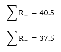
The test statistic itself is the absolute value of the smaller of the above values; in this case, we get T = 37.5. In the table, the critical value for n = 12 and α = 0.05 for a two-tailed test is 13. Since T > 13, we fail to reject the null and retain the claim that the population median is, in fact, 8.
Example in R
No R example this week; most of this is easy enough to do by hand for a small-ish sample.
Week 5: The Single-Sample Test for Evaluating Population Kurtosis
Last week we did a test for population skew, which represents the third moment about the mean. Now we’re going to move onto the fourth moment by doing a single-sample test to evaluate population kurtosis!
When Would You Use It?
The test of population kurtosis test is a parametric test used in a single sample situation to assess if a sample originates from a population that is mesokurtic (as opposed to leptokurtic or platykurtic).
What Type of Data?
The test for kurtosis requires interval or ratio data.
Test Assumptions
None listed.
Test Process
Step 1: Formulate the null and alternative hypotheses. The null hypothesis claims that the kurtosis parameter γ2 in the population is equal to 0, which corresponds to a mesokurtic distribution; the alternative hypothesis claims otherwise (the population kurtosis parameter is greater than, less than, or not equal to the value specified in the null hypothesis, suggesting a leptokurtic or platykurtic distribution).
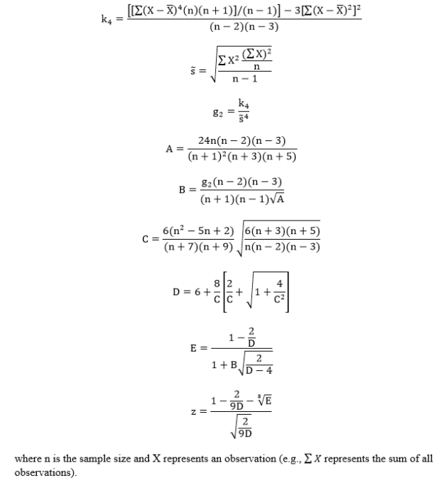
Step 2: Compute the test statistic value, a z-score. The test statistic requires several calculations to be obtained. The calculations are as follows:
Step 3: Obtain the p-value associated with the calculated chi-square. The p-value indicates the probability of observing a test statistic as extreme or more extreme than the observed test statistic, under the assumption that the null hypothesis is true.
Step 4: Determine the conclusion. If the p-value is larger than the prespecified α-level, fail to reject the null hypothesis (that is, retain the claim that the population distribution is mesokurtic). If the p-value is smaller than the prespecified α-level, reject the null hypothesis in favor of the alternative.
Example
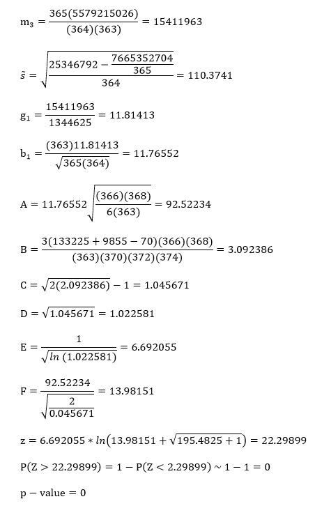
The data for this example come from my n = 365 song downloads from 2010. I want to create a hypothesis test regarding the kurtosis of the distribution of song lengths (in seconds).
H0: γ2 = 0
Ha: γ2 0
Set α = 0.05.
Computations:
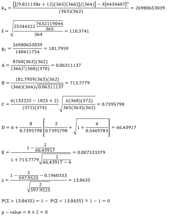
Since our p-value is basically zero, it is smaller than our alpha-level, and we reject H0 and claim that the population is not mesokurtic (γ2 ≠ 0).
Example in R
dat = read.table('clipboard',header=T) #'dat' is the name of the imported raw data
n = length(dat)
xbar = mean(dat)
k = ((((sum((dat-xbar)^4))*n*(n+1))/(n-1))-(3*((sum((dat-xbar)^2))^2)))/((n-2)*(n-3))
s = sqrt(((sum(dat^2))-(((sum(dat))^2)/n))/(n-1))
g2 = k/(s^4)
A = (24*n*(n-2)*(n-3))/(((n+1)^2)*(n+3)*(n+5))
B = (g2*(n-2)*(n-3))/((n-1)*(n+1)*sqrt(A))
C = ((6*((n^2)-(5*n)+2))/((n+7)*(n+9)))*sqrt((6*(n+3)*(n+5))/(n*(n-2)*(n-3)))
D = 6+(8/C)*((2/C)+sqrt(1+(4/(C^2))))
E = (1-(2/D))/(1+(B*sqrt(2/(D-4))))
z = (1-(2/(9*D))-((E)^(1/3)))/(sqrt(2/(9*D)))      #test statistic
pval = (1-pnorm(z))*2                              #p-value
Week 4: The Single-Sample Test for Evaluating Population Skewness
Last week we did a test for population variance, which represents the second moment about the mean. Today we’re going to go one moment further and do a single-sample test to evaluate population skewness (which represents the third moment about the mean)!
When Would You Use It?
The test of population skewness test is a parametric test used in a single sample situation to determine if a sample originates from a population that is symmetrical (that is, not skewed).
What Type of Data?
The test for skewness requires interval or ratio data.
Test Assumptions
None listed.
Test Process
Step 1: Formulate the null and alternative hypotheses. The null hypothesis claims that the skewness parameter γ in the population is equal to 0, which corresponds to symmetry; the alternative hypothesis claims otherwise (the population skewness parameter is greater than, less than, or not equal to the value specified in the null hypothesis, suggesting there is some skew).
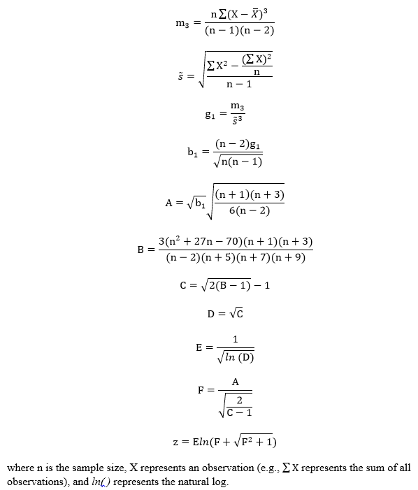
Step 2: Compute the test statistic value, a z-score. The test statistic requires several calculations to be obtained. The calculations are as follows:
Step 3: Obtain the p-value associated with the calculated chi-square. The p-value indicates the probability of observing a skew as extreme or more extreme than the observed sample skew, under the assumption that the null hypothesis is true.
Step 4: Determine the conclusion. If the p-value is larger than the prespecified α-level, fail to reject the null hypothesis (that is, retain the claim that there is symmetry (no skew) in the population). If the p-value is smaller than the prespecified α-level, reject the null hypothesis in favor of the alternative.
Example
As in the last test, the data for this example come from my n = 365 song downloads from 2010. I want to create a hypothesis test regarding the skew of the distribution of song lengths (in seconds). Based on the following histogram, I’m going to say that this distribution has a right skew.

Thus,
H0: γ = 0
Ha: γ > 0
Set α = 0.05.
Computations:
Since our p-value is basically zero, it is smaller than our alpha-level, and we reject H0 and claim that the population is indeed positively skewed (γ > 0)
Example in R
dat = read.table('clipboard',header=T) #'dat' is the name of the imported raw data
hist(dat)                              #creates histogram of data
n = 365
m3 =(n*sum((dat-mean(dat))^3))/((n-1)*(n-2))
s3 = sqrt((sum(dat^2)-(((sum(dat))^2)/n))/(n-1))
g1 = m3/(s3)^3
b1 = ((n-2)*g1)/(sqrt(n*(n-1)))
A = b1*sqrt(((n+1)*(n+3))/(6*(n-2)))
B = (3*((n^2)+(27*n)-70)*(n+1)*(n+3))/((n-2)*(n+5)*(n+7)*(n+9))
C = sqrt(2*(B-1))-1
D = sqrt(C)
E = 1/sqrt((log(D)))
F = A/(sqrt(2/(C-1)))
z = E*log(F+sqrt((F^2)+1))            #test statistic
pval = (1-pnorm(z))                   #p-value
Week 3: The Single-Sample Chi-Square Test for a Population Variance
Today we’re going to move away from testing for means and do the single-sample chi-square test for a population variance!
When Would You Use It?
The chi-square test is a parametric test used in a single sample situation to determine if a sample originates from a population with a specific variance σ2.
What Type of Data?
The chi-square test for variance requires interval or ratio data.
Test Assumptions
- The sample is a simple random sample from the population of interest.
- The distribution underlying the data is normal.
Test Process
Step 1: Formulate the null and alternative hypotheses. The null hypothesis claims that the variance in the population is equal to a specific value; the alternative hypothesis claims otherwise (the population variance is greater than, less than, or not equal to the value specified in the null hypothesis.
Step 2: Compute the chi-square value. The chi-square value is computed as follows:

Step 3: Obtain the p-value associated with the calculated chi-square. The p-value indicates the probability of observing a sample variance as extreme or more extreme than the observed sample variance, under the assumption that the null hypothesis is true.
Step 4: Determine the conclusion. If the p-value is larger than the prespecified α-level, fail to reject the null hypothesis (that is, retain the claim that the variance in the population is equal to the value specified in the null hypothesis). If the p-value is smaller than the prespecified α-level, reject the null hypothesis in favor of the alternative.
Example
The data for this example come from my n = 365 song downloads from 2010. I want to create a hypothesis test regarding the variance of the song lengths (in seconds). I have no idea what the variance is, but I’m going to say that I suspect the variance to be (120)2, or two minutes squared. Set α = 0.05
H0: σ2 = 14,400 seconds
Ha: σ2 ≠ 14,440 seconds
The sample variance is calculated to be 12182.44.
Computations:
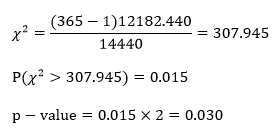
Since our p-value is smaller than our alpha-level, we reject H0 and claim that the population variance is greater than (120)2 seconds.
Example in R
dat=read.table('clipboard',header=T) #'dat' is the name of the imported raw data
sigma = 120^2
s = var(dat)
n = 365
chisq = ((n-1)*s)/(sigma)  #chi-square value
pval = (pchisq(chisq, n-1))*2    #p-value
                                 #n-1 is the degrees of freedom
Week 2: The Single-Sample t Test
Today we’ll be discussing another commonly used statistical test—one that is highly related to last week’s test: the single-sample t test!
When Would You Use It?
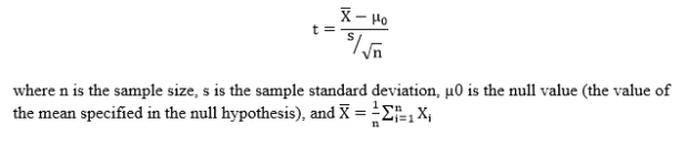
The single-sample t test is a parametric test used in a single sample situation to determine if the sample originates from a population with a specific mean µ. This test is used when the population standard deviation, σ, is not known (it must be estimated with the sample standard deviation, s).
What Type of Data?
The single-sample t test requires interval or ratio data.
Test Assumptions
- The sample is a simple random sample from the population of interest.
- The distribution underlying the data is normal.
Test Process
Step 1: Formulate the null and alternative hypotheses. The null hypothesis claims that the mean in the population is equal to a specific value; the alternative hypothesis claims otherwise (the population mean is greater than, less than, or not equal to the value specified in the null hypothesis.
Step 2: Compute the t-score. The t-score is computed as follows:
Step 3: Obtain the p-value associated with the calculated t-score. The p-value indicates the probability of observing a sample mean as extreme or more extreme than the observed sample mean, under the assumption that the null hypothesis is true.
Step 4: Determine the conclusion. If the p-value is larger than the prespecified α-level, fail to reject the null hypothesis (that is, retain the claim that the mean in the population is equal to the value specified in the null hypothesis). If the p-value is smaller than the prespecified α-level, reject the null hypothesis in favor of the alternative.
Example
The data for this example are the recorded mileages of my n = 306 walks from 2015. Mileage is recorded to the second decimal place. Since there is no real way I can determine what the population standard deviation should be, I will estimate it with the sample standard deviation, and thus must use a t test for a test of the mean value. I’m going to guess that my average walk is greater than 7 miles, ‘cause I honestly can’t remember what the actual average was, but I’m pretty sure it was more than 7. Set α = 0.05.
H0: µ = 7 miles
Ha: µ > 7 miles
The sample mean is calculated to be 8.246 and the sample standard deviation is calculated to be 4.429
Computations:

Since our p-value is much smaller than our alpha-level, we reject H0 and claim that the population mean is greater than 7 miles.
Example in R
dat=read.table('clipboard',header=T) #'dat' is the name of the imported raw data
mu = 7
s = sd(dat)
n = 306
xbar = mean(dat)
t = (xbar-mu)/(s/sqrt(n))  #t-score
pval = (1-pt(t, n-1))*2          #p-value
                                 #n-1 is the degrees of freedom
Week 1: The Single-Sample z Test
Today we’ll be discussing one of the most commonly used statistical tests and one of the first ones taught in introductory stats: the single-sample z test!
When Would You Use It?
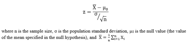
The single-sample z test is a parametric test used in a single sample situation to determine if the sample originates from a population with a specific mean µ. This test is used when the population standard deviation, σ, is known.
What Type of Data?
The single-sample z test requires interval or ratio data.
Test Assumptions
- The sample is a simple random sample from the population of interest.
- The distribution underlying the data is normal.
Test Process
Step 1: Formulate the null and alternative hypotheses. The null hypothesis claims that the mean in the population is equal to a specific value; the alternative hypothesis claims otherwise (the population mean is greater than, less than, or not equal to the value specified in the null hypothesis.
Step 2: Compute the z-score. The z-score is computed as follows:
Step 3: Obtain the p-value associated with the calculated z-score. The p-value indicates the probability of observing a sample mean as extreme or more extreme than the observed sample mean, under the assumption that the null hypothesis is true.
Step 4: Determine the conclusion. If the p-value is larger than the prespecified α-level, fail to reject the null hypothesis (that is, retain the claim that the mean in the population is equal to the value specified in the null hypothesis). If the p-value is smaller than the prespecified α-level, reject the null hypothesis in favor of the alternative.
Example
The data for this example are n = 400 IQ scores from random sample of individuals ages 18 to 87. The test used to obtain the scores was constructed similar to the Stanford-Binet IQ test, meaning that we can assume that the average IQ score in the population should be 100 and the population standard deviation σ is known and is equal to 15. Let’s test the claim that the population mean is actually different than 100. Set α = 0.05.
H0: µ = 100
Ha: µ ≠ 100
The sample mean is calculated to be 101.864
Computations:
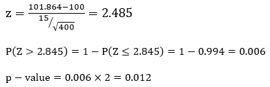
Since our p-value is smaller than our alpha-level (0.012 > 0.05), we reject H0 and claim that the population mean is different from 100.
Example in R
dat=read.table('clipboard',header=T) #'dat' is the name of the imported raw data
mu = 100
sigma = 15
n = 400
xbar = mean(dat)
z = (xbar-mu)/(sigma/sqrt(n))  #z-score
pval = (1-pnorm(z))*2          #p-value
                               #pnorm calculates the left-hand area
                               #multiply by two because it is a two-sided test
Statistics Sunday: An Introductory Post
Every Sunday of this year, I plan on focusing on one of the statistical tests featured in the Handbook of Parametric and Nonparametric Statistical Procedures (5th edition) by David J. Sheskin. I will include the following information in each post:
- When would you use the test? What type of research question might the test help to answer?
- For what type of data is the test appropriate? Do you need interval/ratio data, categorical data, etc.?
- Assumptions. What assumptions must be met in order for the test to be accurately employed?
- Process. The steps (and equations) of the test.
- Example. The test carried out with real data.
- Example in R. The R code for the above example.
I’ll start this tomorrow, and while I’ll probably put a little menu button up at the top of my blog homepage to link to all the tests (a thing like a “Statistics Sundays” button or whatnot), I figured I should explain it here, too.
YAY!
More Stats Planning
HEY PEEPS!
I typed out all the tests from my statistical tests handbook, then narrowed them down to 52 that I want to feature, one per week, on my blogs next year. Check ‘em:
- Week 1: The Single-Sample z Test
- Week 2: The Single-Sample t Test
- Week 3: The Single-Sample Chi-Square Test for a Population Variance
- Week 4: The Single-Sample Test for Evaluating Population Skewness
- Week 5: The Single-Sample Test for Evaluating Population Kurtosis
- Week 6: The Wilcoxon Signed-Ranks Test
- Week 7: The Kolmogorov-Smirnov Goodness-of-Fit Test for a Single Sample
- Week 8: The Chi-Square Goodness-of-Fit Test
- Week 9: The Binomial Sign Test for a Single Sample
- Week 10: The z Test for a Population Proportion
- Week 11: The Single-Sample Runs Test
- Week 12: The t Test for Two Independent Samples
- Week 13: F Test for Two Population Variances
- Week 14: The Median Absolute Deviation Test for Identifying Outliers
- Week 15: The Mann-Whitney U Test
- Week 16: The Kolmogorov-Smirnov Test for Two Independent Samples
- Week 17: The Moses Test for Equal Variability
- Week 18: The Siegel-Tukey Test for Equal Variability
- Week 19: The Chi-Square Test for Homogeneity
- Week 20: The Chi-Square Test of Independence
- Week 21: The z Test for Two Independent Proportions
- Week 22: The t Test for Two Dependent Samples
- Week 23: The Wilcoxon Matched-Pairs Signed-Ranks Test
- Week 24: The Binomial Sign Test for Two Dependent Samples
- Week 25: The McNemar Test
- Week 26: The Single-Factor Between-Subjects Analysis of Variance
- Week 27: The Kruskal-Wallis One-Way Analysis of Variance by Ranks
- Week 28: The van der Waerden Normal-Scores Test for k Independent Samples
- Week 29: The Single-Factor Within-Subjects Analysis of Variance
- Week 30: The Friedman Two-Way Analysis of Variance by Ranks
- Week 31: The Cochran Q Test
- Week 32: The Between-Subjects Factorial Analysis of Variance
- Week 33: Analysis of Variance for a Latin Square Design
- Week 34: The Within-Subjects Factorial Analysis of Variance
- Week 35: The Pearson Product-Moment Correlation Coefficient
- Week 36: The Point-Biserial Correlation Coefficient
- Week 37: The Biserial Correlation Coefficient
- Week 38: The Tetrachoric Correlation Coefficient
- Week 39: Spearman’s Rank-Order Correlation Coefficient
- Week 40: Kendall’s Tau
- Week 41: Kendall’s Coefficient of Concordance
- Week 42: Goodman and Kruskal’s Gamma
- Week 43: Multiple Regression
- Week 44: Hotelling’s T2
- Week 45: Multivariate Analysis of Variance
- Week 46: Multivariate Analysis of Covariance
- Week 47: Discriminant Function Analysis
- Week 48: Canonical Correlation
- Week 49: Logistic Regression
- Week 50: Principal Components Analysis and Factor Analysis
- Week 51: Path Analysis
- Week 52: Structural Equation Modeling
Yeah. It’ll be fun!
Twiddle
Remember this?
It’s the big book of statistical tests that my mom got me back in like 2012. I didn’t know most of the tests in it at the time (mainly because I hadn’t done my stats-emphasis math degree yet), but now I feel a bit more knowledgeable about its contents.
So what I’d like to do as a resolution for 2016 is go through this book and focus on one test (with examples!) every week in my blog. Maybe on Sundays or something.
I’ll post more on this as it gets closer to the new year, but just a warning. There will be stats.

