Plotting
Aalskdfsdlhfgdsgh, this is super cool.
Today in probability we were talking about the binary expansion of decimal fractions—in particular, those in the interval [0,1).
Q: WTF is the binary expansion of a decimal fraction?
A: If you know about binary in general, you know that to convert a decimal number like 350 to binary, you have to convert it to 0’s and 1’s based on a base-2 system (20, 21, 22, 23, 24, …). So 350 = 28 + (0*27) + 26 + (0*25) + 24 + 23 + 22 + 21 + (0*20) = 101011110 (1’s for all the “used” 2k’s and 0’s for all the “unused” 2k’s).
It’s the same thing for fractions, except now the 2k’s are 2-k‘s: 1/21, 1/22, 1/23, …).
So let’s take 5/8 as an example fraction we wish to convert to binary. 5/8 = 1/21 + (0*1/22) + 1/23, so in binary, 5/8 = 101. Easy!*
So we used this idea of binary expansion to talk about the Strong Law of Large Numbers for the continuous case (rather than the discrete case, which we’d talked about last week), but then we did the following:

where x = 0.x1 x2 x3 x4… is the unique binary expansion of x containing an infinite number of zeros.
Dr. Chen asked us to, as an exercise, plot γ1(x), γ2(x), and γ3(x) for all x in [0,1). That is, plot what the first, second, and third binary values look like (using the indicator function above) for all decimal fractions in [0,1).
We could do this by hand (it wasn’t something we had to turn in), but I’m obsessive and weird, so I decided to write some R code to do it for me (and to confirm what I got by hand)!
Code:
x = seq(0, 1, by = .0001)
x = sort(x)
n = length(x)
y = matrix(NaN, n)
z = matrix(NaN, n)
bi = matrix(NaN, n, nrow=n, ncol=3)

for (i in 1:n) {
   pos1 = trunc(x[i]*2)
   if (pos1 == 0) {
      bi[i,1] = 1
      y[i] = x[i]*2
      }
   else if (pos1 == 1) {
      bi[i,1] = -1
      y[i] = -1*(1-(x[i]*2))
      }
   pos2 = trunc(y[i]*2)
   if (pos2 == 0) {
      bi[i,2] = 1
      z[i] = y[i]*2
      }
   else if (pos2 == 1) {
      bi[i,2] = -1
      z[i] = -1*(1-(y[i]*2))
      }
   pos3 = trunc(z[i]*2)
   if (pos3 == 0) {
      bi[i,3] = 1
      }
   else if (pos3 == 1) {
      bi[i,3] = -1
      }
   }

bin = cbind(x,bi)
bin = as.matrix(bin)
plot(bin[,1],bin[,2],  type = 'p', col = 'black', lwd = 7,
     ylim = c(-1, 1), xlim = c(0, 1), xlab = "Value",
     ylab = "Indicator Value",
     main = "Indicator Value vs. Value on [0,1) Interval")
lines(bin[,1],bin[,3], type='p', lwd = 4, col='green')
lines(bin[,1],bin[,4], type='p', lwd = .25, col='red')
Results:

(black is 1/2, green is 1/4, red is 1/8)
I tried to make the plot readable so that you could see the overlaps. Not sure if it works.
Makes sense, though. Until you get to ½, you can’t have a 1 in that first expansion place, since 1 represents the value 1/21. Once you get past ½, you need that 1 in the first expansion place. Same things with 1/22 and 1/23.
SUPER COOL!
(I love R.)
*Note that this binary expression is not unique. All the work we did in class was done under the assumption that we were using the expressions that had an infinite number of zeroes rather than an infinite number of ones.
“How Long Have You Been Waiting for the Bus?” IT DOESN’T MATTER!
Today I’m going to talk about probability!
YAY!
Suppose you just went grocery shopping and are waiting at the bus stop to catch the bus back home. It’s Moscow and it’s November, so you’re probably cold, and you’re wondering to yourself what the probability is that you’ll have to wait more than, say, two more minutes for the bus to arrive.
How do we figure this out? Well, the first thing we need to know is that things like wait time are usually modeled as exponential random variables. Exponential random variables have the following pdf:
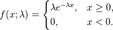
where lambda is what’s usually called the “rate parameter” (which gives us info on how “spread out” the corresponding exponential distribution is, but that’s not too important here). So let’s say that for our bus example, lambda is, hmm…1/2.
Now we can figure out the probability that you’ll be waiting more than two minutes for the bus. Let’s integrate that pdf!
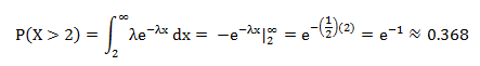
So you have a probability of .368 of waiting more than two minutes for the bus.
Cool, huh? BUT WAIT, THERE’S MORE!
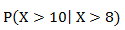
Now let’s say you’ve waited at the bus stop for eight whole minutes. You’re bored and you like probability, so you think, “what’s the probability, given that I’ve been standing here for eight minutes now, that I’ll have to wait at least 10 minutes total?”
In other words, given that the wait time thus far has been eight minutes, what is the probability that the total wait time will be at least 10 minutes?
We can represent that conditional probability like this:
And this can be found as follows:
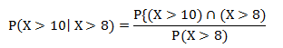
Which can be rewritten as:
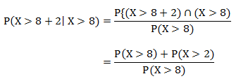
Which is, using the same equation and integration as above:
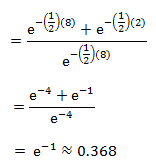
Which is the exact same probability as the probability of having to wait more than two minutes (as calculated above)!
WOAH, MIND BLOWN, RIGHT?!
This is a demonstration of a particular property of the exponential distribution: that of memorylessness. That is, if we select an arbitrary point s along an exponential distribution, the probability of observing any value greater than that s value is exactly the same as it would be if we didn’t even bother selecting the s. In other words, the distribution of the remaining function does not depend on s.
Another way to think about it: suppose I have an alarm clock that will go off after a time X (with some rate parameter lambda). If we consider X as the “lifetime” of the alarm, it doesn’t matter if I remember when I started the clock or not. If I go away and come back to observe the alarm hasn’t gone off, I can “forget” about the time I was away and still know that the distribution of the lifetime X is still the same as it was when I actually did set the clock, and will be the same distribution at any time I return to the clock (assuming it hasn’t gone off yet).
Isn’t that just the coolest freaking thing?! This totally made my week.
“When Will I Use That?” – Calculus Edition
Alternate title: Claudia Makes Things Way More Complicated than They Need to Be Because She Sucks
We had this bonus question on our homework for Probability today:
Suppose X has a density defined by

Let FX(x) be the cumulative distribution of X. Find the area of the region bounded by the x-axis, the y-axis, the line y = 1, and the curve y = FX(x).
And I was like, “Aw, sweet! Areas of regions! CALCULUS!”
So first, I had to find the cumulative distribution function (cdf) of X. Easy. It’s just the integral of the density fX(x) from negative infinity to a constant b. In this case:

With 2 ≤ b ≤ 3. So that’s my curve y. The area I’m looking for, therefore, is this (the red part, not the purplish part):

Now anyone with half a brain would look at this and go, “oh yeah, that’s easy. I can find the area of the rectangle formed by the two axes, the line y = 1, and the line x = 3, then find the area of the region below the curve from 2 to 3, and subtract the latter from the former to get the correct area.”
Which works. Area of rectangle = 3, area of region below FX(x) = .25, area of region of
interest = 2.75.
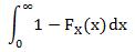
Or they could remember the freaking formula that was explicitly taught last week. Such areas can be calculated using:
But did I see either of those? Nooooooope.
I looked at the graph and was like, “how the hell do you find that?” I tried a few things that didn’t work, then realized that it would be a lot easier to figure out if I changed the integral from being in terms of x (or b, rather) to being in terms of y.
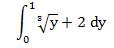
So then I just had to integrate. This gave me the right answer: 2.75!
Moral of the story: don’t complicate things. But if you do complicate things, you might actually end up in a scenario where you’ll use something that you were taught back in calculus I but didn’t ever suspect you’d actually use. I had appreciated learning the handy-dandy technique of changing variables, but I didn’t think I’d be in a situation where I’d apply it. Shows what I know, eh?
It was a nice refresher, at least. I’ve missed calculus.
I think I’m a witch, guys
Remember that whole creepy-beating-the-odds thing with the 13-digit number last week? Well today my TA returned a stack of homeworks to me so I brought them to my office and started in on alphabetizing them. This involved splitting the big pile into two smaller ones. So I attempt to do that, but it turns out that the unsorted pile was actually naturally divided into two sections: the first containing last names starting with A – L, the other containing last names starting with M – Z.
Which is creepy on its own.
So I go through the A – L pile and alphabetize, then I go on to the M – Z pile. Well, guess what?
IT WAS ALREADY ALPHABETIZED.
Please keep I mind that my TA does not attempt to alphabetize the homeworks as he grades and has told me that he usually grades them in the order they are in the original pile I hand him.
So yeah.
Creepy stuff, man.
What are the odds?
Holy freaking crap, you guys.
HOLY. FREAKING. CRAP.
I beat some incredibly ridiculous odds today.
I was in the library this afternoon writing my lecture. This week we’re talking about random variables, so I wanted to create an example of both a discrete random variable and a continuous random variable. I wanted to show that a continuous variable can take on ANY value in a given interval, so I decided to just mash the number pad on the keyboard to come up with a number with a bunch of decimals. So I mashed away and got this: 128.3671345993.
Satisfied with this as an example, I turned the page in our textbook to keep working. And what was the book’s example for a continuous variable? 128.3671345993.
WHAT.
What the hell are the odds of that? (0.0000000001:1 discounting the decimal point).
Ridiculous odds are ridiculous. I had a little heart attack in the library.
This Week’s Science Blog: What are the Odds?
A recent study has shown that babies as young as twelve months old have a basic understanding of probability.
How did researchers come to this conclusion? They ran a bunch of twelve- and fourteen-month-olds through a series of tests. First, they gave the babies both a black and a pink lollipop and recorded the preference of the baby. Once the preference was recorded, the babies were let go and then brought back at a later date for a second test.
The second test involved showing the babies two clear jars—one of which contained many pink lollipops and only a few black ones, the other containing many black lollipops but few pink ones. With the babies still watching, a researcher reached a hand into each jar and pulled out a lollipop, but concealed with their hand the color of the candy. They dropped the lollipops into separate opaque cups so that the babies still couldn’t see the color, then asked them to choose one of the cups.
The cool thing? The babies consistently chose the cup belonging to the more “likely” jar. That is, they selected the cup that belonged to the candy drawn from the jar containing the greatest number of the babies’ preferred lollipop color. From the article, “this indicates that many kids, even when they’re very young, are able to make the mental connection that a random lollipop picked from a jar that had more pink lollipops, is more likely to be pink than one picked from a jar containing mostly black lollipops.”
How cool is that?
Probability in Action!
I LOVE these things.

