HELLO, DUDES!

Sit back, relax, and tune your mind to the statistics channel, as today I’m going to blog about the Central Limit Theorem!

What is the Central Limit Theorem? Here’s a simple explanation: take a random sample from a distribution—any distribution—and calculate that sample’s mean. Do this with a bunch of independent samples from that same distribution. As the number of samples increases, the distribution of those sample’s means will approximate a normal distribution, regardless of the shape of the distribution from which the samples were drawn. That is, the sample means will be approximately normally distributed no matter what distribution the samples are from.

ILLUSTRATION TIME!

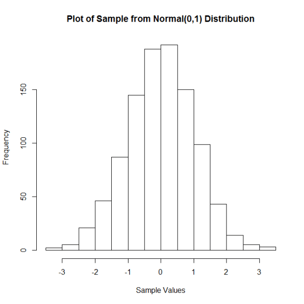
Let’s start with samples from a standard normal distribution, with mean = 0 and standard deviation = 1. Here is a histogram of a sample of 100 observations (n = 100) from this distribution.

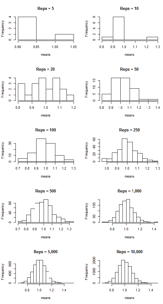
Now I’m going to do the following: I’m going to take a certain number (let’s call them “reps”) of samples of size n = 100, calculate the corresponding sample means, and then plot said means. I’m going to do this for 5, 10, 20, 50, 100, 250, 500, 1,000, 5,000, and 10,000 reps of samples of size n = 100. Then I’m going to plot the sample means. The following plots show the results:

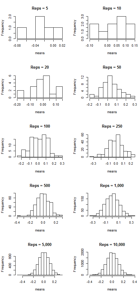
Notice that as the number of samples (the “reps”) increases, the distribution of sample means resembles more and more a normal distribution centered at mean = 0. That suggests that the more samples we take, the more the means “cluster” around the true mean, which in this case is zero.

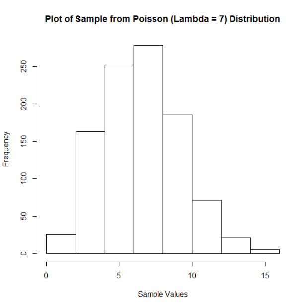
But this doesn’t just work with normal-shaped distributions! Let’s do the same thing, but now by taking samples from a Poisson distribution with lambda = 7. Here is the histogram of a sample of 100 observations (n = 100) from this distribution:

Not quite normal, huh? But look what happens with the means when we employ the same technique as we did above:

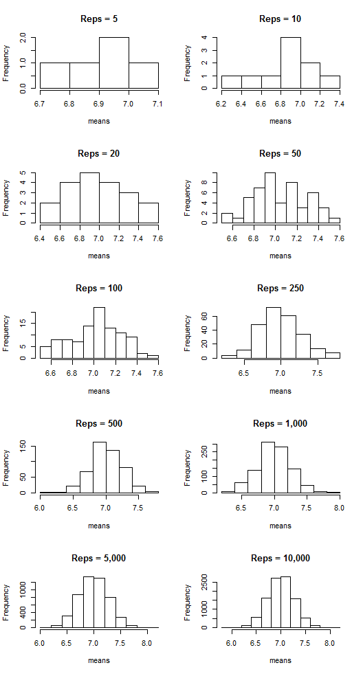
The sample means are clustering around the lambda value, 7, and appear more and more normal-shaped as the number of reps increases.

Want a few more examples?

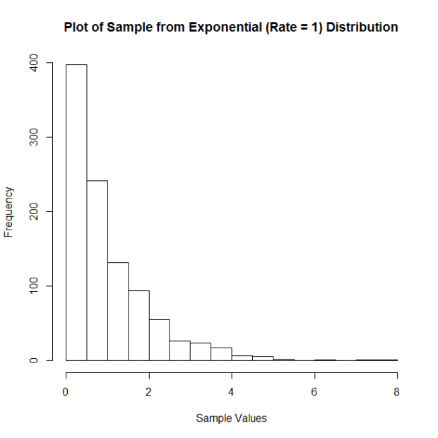
Let’s take samples from an exponential distribution with rate parameter = 1. Here is the histogram of a sample of 100 observations (n = 100) from this distribution:

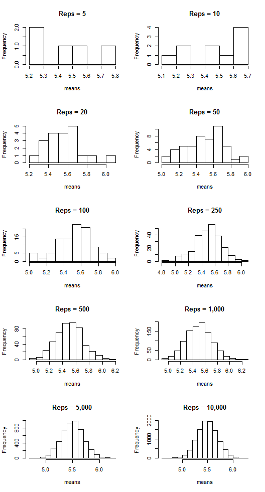
And the plots of the means:

What about samples from a uniform distribution ranging from 2 to 9. Here is the histogram of a sample of 100 observations (n = 100) from this distribution:

And the means:

COOL, HUH??? It’s the CLT in action!